Your handwritten-digit classifier reports 96% and you ship it. But a single accuracy number hides everything that matters: a layer whose filters are all dead, a nonlinearity pinned in saturation, inputs that were never normalized, a handful of flipped labels quietly capping the score. Feature maps — the activations flowing inside the network — turn that black box transparent. This article trains a small CNN on MNIST[1] with PyTorch[2], then deliberately breaks it six different ways — using nothing but forward hooks and a plotting library to make each bug visible before it silently ruins your model.
{readmore}Setup
python -m venv .venv
.venv\Scripts\activate            # Windows
pip install -r requirements.txt   # torch, torchvision, matplotlib, numpy, pillow

# For an NVIDIA GPU, install the CUDA build of PyTorch instead:
pip install torch torchvision --index-url https://download.pytorch.org/whl/cu126
Line 1 creates the virtual environment; line 2 activates it on Windows; line 3 installs the CPU dependencies — PyTorch, torchvision[3] for MNIST, and Matplotlib[4] for the plots; lines 5–6 are the alternative one-line install of the CUDA build for an NVIDIA GPU. Everything below runs on the GPU when one is available and falls back to the CPU otherwise:
import torch

def pick_device():
    return torch.device("cuda" if torch.cuda.is_available() else "cpu")
Line 1 imports torch; lines 3–4 define pick_device(), returning a CUDA device when one is available and the CPU otherwise.
Capturing feature maps with forward hooks
The whole technique rests on one PyTorch feature: a forward hook lets you read a layer's output every time it runs, without editing the model. First, a small CNN whose activation and batch-norm are knobs, so the same class can produce the healthy baseline and every broken variant:
import torch
from torch import nn

class Small_CNN(nn.Module):
    def __init__(self, num_classes=10, activation="relu", use_bn=True, init="kaiming"):
        super().__init__()
        def block(in_ch, out_ch, pool):
            layers = [nn.Conv2d(in_ch, out_ch, kernel_size=3, padding=1)]
            if use_bn:
                layers.append(nn.BatchNorm2d(out_ch))
            layers.append(make_activation(name=activation))
            if pool:
                layers.append(nn.MaxPool2d(2))
            return nn.Sequential(*layers)

        self.conv1 = block(in_ch=1, out_ch=16, pool=True)     # 28 -> 14
        self.conv2 = block(in_ch=16, out_ch=32, pool=True)    # 14 -> 7
        self.conv3 = block(in_ch=32, out_ch=64, pool=False)   # 7  -> 7
        self.pool = nn.AdaptiveAvgPool2d(1)
        self.classifier = nn.Linear(64, num_classes)
        self.apply_init(scheme=init)

    def feature_layers(self):
        return {"conv1": self.conv1, "conv2": self.conv2, "conv3": self.conv3}

    def forward(self, x):
        x = self.conv1(x)
        x = self.conv2(x)
        x = self.conv3(x)
        x = torch.flatten(self.pool(x), 1)
        return self.classifier(x)
Lines 1–2 import PyTorch. Lines 4–21 define Small_CNN: the block() helper (lines 7–14) stacks a convolution, an optional BatchNorm[5], the chosen activation and an optional max-pool into a Sequential; lines 16–18 build three such blocks (the first two halve the 28×28 map, the third holds it at 7×7); lines 19–20 are the global average pool and the single linear head, and line 21 applies the chosen weight-init scheme. Lines 23–24 expose the three blocks by name — the hook targets — and lines 26–31 are the forward pass. (make_activation() just maps "relu" / "leaky" / "sigmoid" to the matching nn module, and apply_init() applies the named weight-init scheme — "kaiming", "tiny" or "large" — that the broken variants below rely on.)
Now the recorder. It registers one hook per named layer and stashes each output tensor:
class Activation_Recorder:
    def __init__(self, model, layers):
        self.activations = {}
        self._handles = []
        for name, module in layers.items():
            self._handles.append(module.register_forward_hook(self._make_hook(name=name)))

    def _make_hook(self, name):
        def hook(module, inputs, output):
            self.activations[name] = output.detach()
        return hook

    def remove(self):
        for handle in self._handles:
            handle.remove()
Lines 2–6 register a register_forward_hook on every named layer and keep the handles; lines 8–11 build the hook, which stores each layer's detached output under its name (line 10); lines 13–15 detach the hooks afterwards. register_forward_hook[2] is the entire trick — it taps a layer's output without you touching forward(). Running one batch fills the recorder:
device = pick_device()
model = Small_CNN().to(device).eval()
recorder = Activation_Recorder(model=model, layers=model.feature_layers())

images, labels = next(iter(test_loader))
model(images.to(device))                     # one forward pass fills the recorder

conv1_maps = recorder.activations["conv1"]   # (N, 16, 14, 14)
recorder.remove()
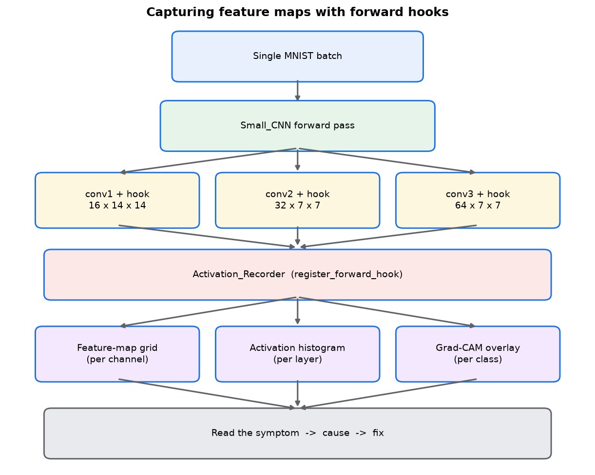
Line 1 picks the device; line 2 builds the model in eval mode; line 3 attaches the recorder to the three conv blocks; line 5 grabs one test batch; line 6 runs a single forward pass, which fires the hooks; line 8 reads conv1's maps — an (N, 16, 14, 14) tensor — and line 9 detaches the hooks. The whole pipeline is summarized in Fig 1.
What a healthy network sees
Before breaking anything, learn what right looks like. Train the baseline (python src/train.py), then plot a few channels of each layer for one test digit:
maps = recorder.activations["conv1"][0]      # first image, 16 channels
fig, axes = plt.subplots(2, 8, figsize=(9, 2.4))
for channel, ax in zip(maps, axes.flat):
    ax.imshow(channel.cpu(), cmap="viridis")
    ax.axis("off")
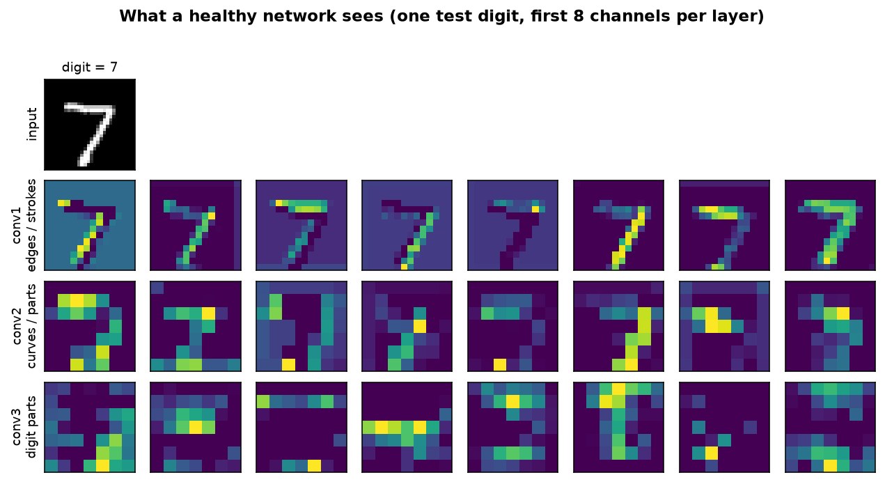
Line 1 takes the 16 channels for the first image; line 2 makes a 2×8 grid; lines 3–5 draw each channel as a small heatmap. The result across all three layers is Fig 2: conv1 fires on strokes and edges, and deeper layers respond to progressively larger parts of the digit. If your first layer already looks like noise, stop — the problem is upstream, in the data, not deep in the model.
Dead and saturated filters
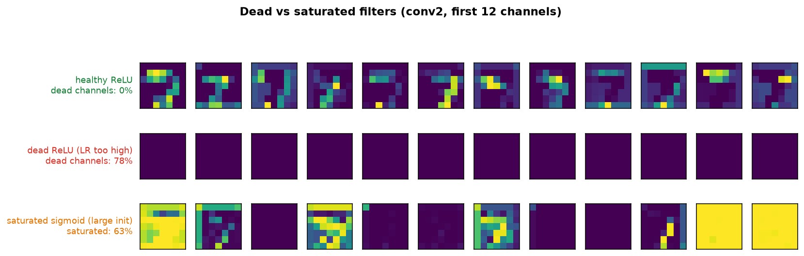
The first failure mode from any feature-map audit: a channel that is entirely blank (all zeros) or entirely flat (pinned at one value). Two classic bugs produce them:
from train import train_model
from model import Small_CNN

# Bug A: a far-too-high learning rate kills ReLU units (dying ReLU)
dead_model, _ = train_model(epochs=2, lr=0.6, use_bn=False, activation="relu")

# Bug B: a large-variance init drives sigmoids straight into saturation
saturated = Small_CNN(activation="sigmoid", use_bn=False, init="large").eval()
Line 5 trains with lr=0.6 and no batch-norm: a couple of oversized gradient steps shove many ReLU pre-activations permanently negative, so those units output zero for every input — the textbook dying ReLU. Line 8 skips training entirely; a standard-deviation-1.0 init already saturates the sigmoids near 0 and 1, where their gradient is almost zero and learning stalls. Recording conv2 for each and comparing to the baseline gives Fig 3. The fix follows the symptom: lower the learning rate, switch to LeakyReLU[6] or ELU[7] so a unit can recover, or re-initialize the weights.
Vanishing and exploding activations
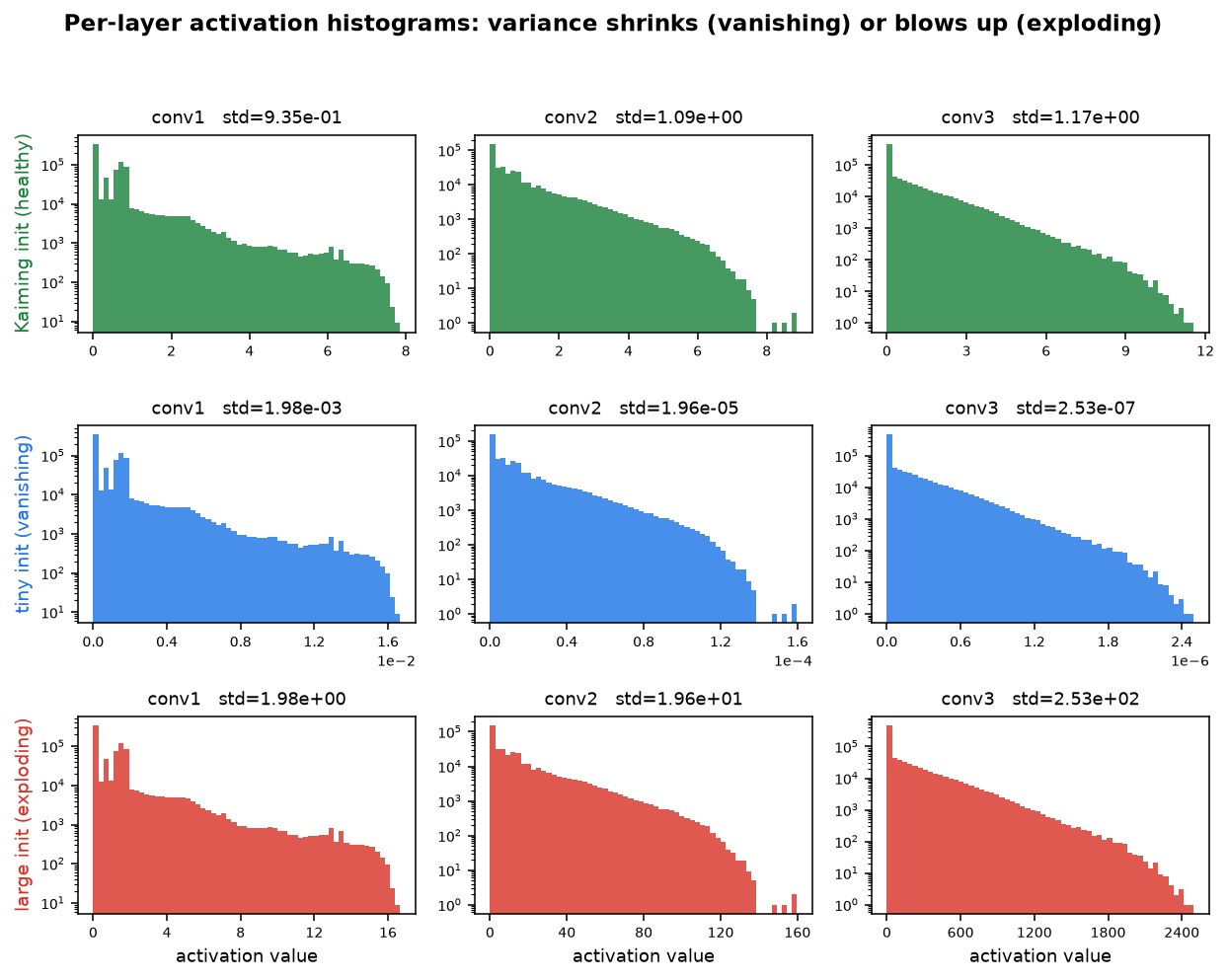
Dead filters are the extreme case; the milder, sneakier version is a distribution that quietly shrinks or grows with depth. Track it by turning batch-norm off (so nothing masks the effect) and printing the spread of each layer's activations under three initializations:
import torch

for init in ("kaiming", "tiny", "large"):
    model = Small_CNN(activation="relu", use_bn=False, init=init).to(device).eval()
    recorder = Activation_Recorder(model=model, layers=model.feature_layers())
    model(images.to(device))
    for name in ("conv1", "conv2", "conv3"):
        values = recorder.activations[name].flatten().cpu()
        print(name, "std =", values.std().item())
    recorder.remove()
Line 3 loops over three initializations; line 4 builds the model with batch-norm off; lines 5–6 hook it and run one batch; lines 7–9 print the standard deviation of each layer's activations; line 10 removes the hooks. The "tiny" init makes the spread collapse toward zero with depth (vanishing); the "large" init makes it blow up (exploding). Plotting those same activations as histograms is Fig 4. The cure is a variance-preserving init — Kaiming[8] for ReLU, Xavier/Glorot[9] for symmetric activations — plus batch-norm.
When preprocessing is the bug
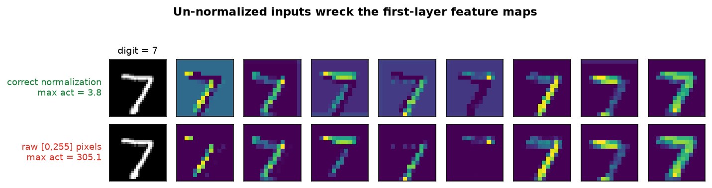
Sometimes the network is fine and the data pipeline is broken. The most common version: forgetting to scale the inputs. Feed the same trained model the same digit, once normalized and once as raw 0–255 pixels:
from torchvision import transforms

MNIST_MEAN, MNIST_STD = (0.1307,), (0.3081,)

correct = transforms.Compose([
    transforms.ToTensor(),                       # [0, 1]
    transforms.Normalize(MNIST_MEAN, MNIST_STD), # ~zero mean, unit std
])

buggy = transforms.Compose([
    transforms.PILToTensor(),                    # [0, 255], never scaled
    transforms.Lambda(lambda t: t.float()),
])
Lines 5–8 are the correct pipeline: ToTensor maps pixels to [0, 1], then Normalize centers them with MNIST's mean and std. Lines 10–13 are the bug: PILToTensor keeps the raw 0–255 integers and only casts them to float, so inputs arrive roughly 100× too large. The same model reads garbage from its first layer — Fig 5. The giveaway is quantitative: the maximum conv1 activation jumps from a handful to the hundreds, exactly the “values 10× higher than expected” smell.
Flipped labels
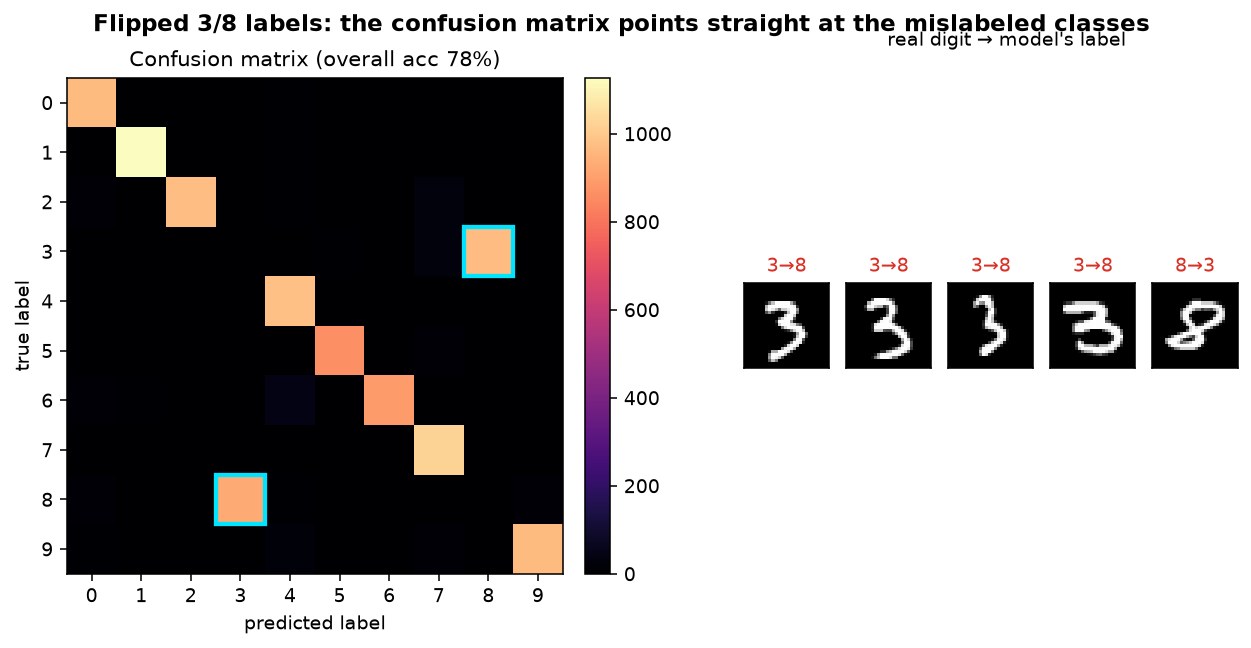
Feature maps also expose label bugs, which no architecture change can fix. Simulate one by swapping two classes in the training set only, then score against the correct test labels and build a confusion matrix:
# swap the 3 and 8 labels in the TRAINING set only
model, history = train_model(epochs=3, flip_labels={3: 8, 8: 3})

matrix = torch.zeros(10, 10, dtype=torch.long)
for images, labels in test_loader:                 # correct test labels
    preds = model(images.to(device)).argmax(1).cpu()
    for t, p in zip(labels, preds):
        matrix[t, p] += 1
Line 2 trains with the 3 and 8 labels swapped in the training set only; lines 4–8 build a 10×10 confusion matrix against the correct test labels. Every real 3 is predicted as 8 and vice-versa, so the matrix lights up off-diagonal at exactly (3, 8) and (8, 3) — Fig 6. That localized, symmetric pattern is the fingerprint of a label bug, not a model that merely struggles to tell two digits apart; the fix is to audit the data pipeline, not the net.
Overfitting in the activations
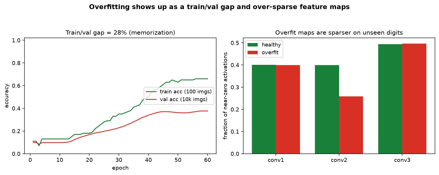
When a model memorizes instead of generalizing, its feature maps grow sparse and overly selective — high for a few remembered examples, near-zero elsewhere. Force it by training on a tiny subset and watch both the accuracy gap and the activation sparsity:
# train on only 100 images for many epochs
model, history = train_model(epochs=60, lr=0.05, subset_size=100)

print(history["train_acc"][-1], history["val_acc"][-1])   # near-1.0 train, lower val

recorder = Activation_Recorder(model=model, layers=model.feature_layers())
model(images.to(device))                                  # unseen test batch
sparsity = (recorder.activations["conv3"].abs() <= 1e-4).float().mean()
recorder.remove()
Line 2 trains on just 100 images for 60 epochs; line 4 shows the tell-tale gap — near-perfect training accuracy, much lower validation accuracy; lines 6–8 measure how much of the last conv layer sits near zero on an unseen batch. The memorizing model is markedly sparser than the baseline, as Fig 7 shows. The accuracy curve tells you that it overfit; the activations tell you how — and warn you when dropout or weight decay is set so hard the maps collapse the other way.
Architecture smells: checkerboard artifacts
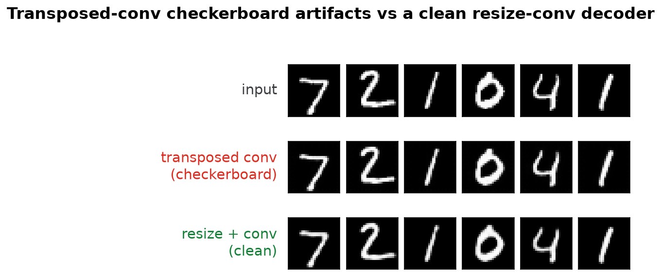
Feature maps validate architecture too. The classic example lives in decoders and GANs: a regular grid stamped onto the output by a transposed convolution whose kernel size is not divisible by its stride. Here are the buggy decoder and its fix, from an MNIST autoencoder:
from torch import nn

# Bug: kernel_size (3) is not divisible by stride (2) -> uneven overlap
checkerboard = nn.Sequential(
    nn.ConvTranspose2d(32, 16, kernel_size=3, stride=2, padding=1, output_padding=1),
    nn.ReLU(inplace=True),
    nn.ConvTranspose2d(16, 1, kernel_size=3, stride=2, padding=1, output_padding=1),
    nn.Sigmoid(),
)

# Fix: upsample by resizing, then convolve
clean = nn.Sequential(
    nn.Upsample(scale_factor=2, mode="nearest"),
    nn.Conv2d(32, 16, kernel_size=3, padding=1), nn.ReLU(inplace=True),
    nn.Upsample(scale_factor=2, mode="nearest"),
    nn.Conv2d(16, 1, kernel_size=3, padding=1), nn.Sigmoid(),
)
Lines 4–9 are the buggy decoder: because each ConvTranspose2d has a kernel size (3) that the stride (2) does not divide evenly, neighbouring output pixels get different amounts of overlap, stamping a regular grid onto the image[10]. Lines 12–17 fix it by splitting the two jobs apart — nearest-neighbour Upsample enlarges the map, then a plain Conv2d fills in detail. Fig 8 puts the two reconstructions side by side.
Grad-CAM: which pixels drove the class
Raw feature maps show what a filter responds to; Grad-CAM answers the dual question — which pixels pushed the model toward its decision. It is a few lines built from the same hooks, a forward hook for the activations and a backward hook for their gradients:
def grad_cam(model, target_layer, image, class_idx=None):
    activation, gradient = {}, {}
    f = target_layer.register_forward_hook(lambda m, i, o: activation.setdefault("v", o))
    b = target_layer.register_full_backward_hook(lambda m, gi, go: gradient.setdefault("v", go[0]))

    scores = model(image)
    class_idx = class_idx or int(scores.argmax(1))
    model.zero_grad()
    scores[0, class_idx].backward()

    weights = gradient["v"][0].mean(dim=(1, 2))          # one weight per channel
    cam = torch.relu((weights[:, None, None] * activation["v"][0]).sum(0))
    f.remove(); b.remove()
    return cam / cam.max(), class_idx
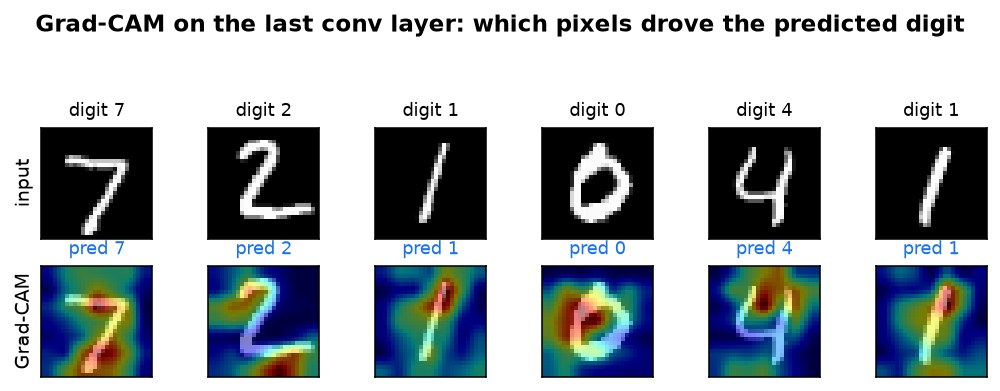
Lines 3–4 register a forward hook (to catch the last conv layer's activations) and a full-backward hook (to catch the gradients flowing into them); lines 6–9 run the forward pass, pick the predicted class, and backpropagate just that score; line 11 averages each channel's gradient into a single importance weight; line 12 takes the ReLU of the weighted sum of activations — the Grad-CAM[11] map; line 13 detaches the hooks; line 14 normalizes and returns it. Overlaid on each digit, it is Fig 9 — the heat sits on the strokes that define each digit, a quick sanity check that the model looks at the right pixels.
A debugging workflow
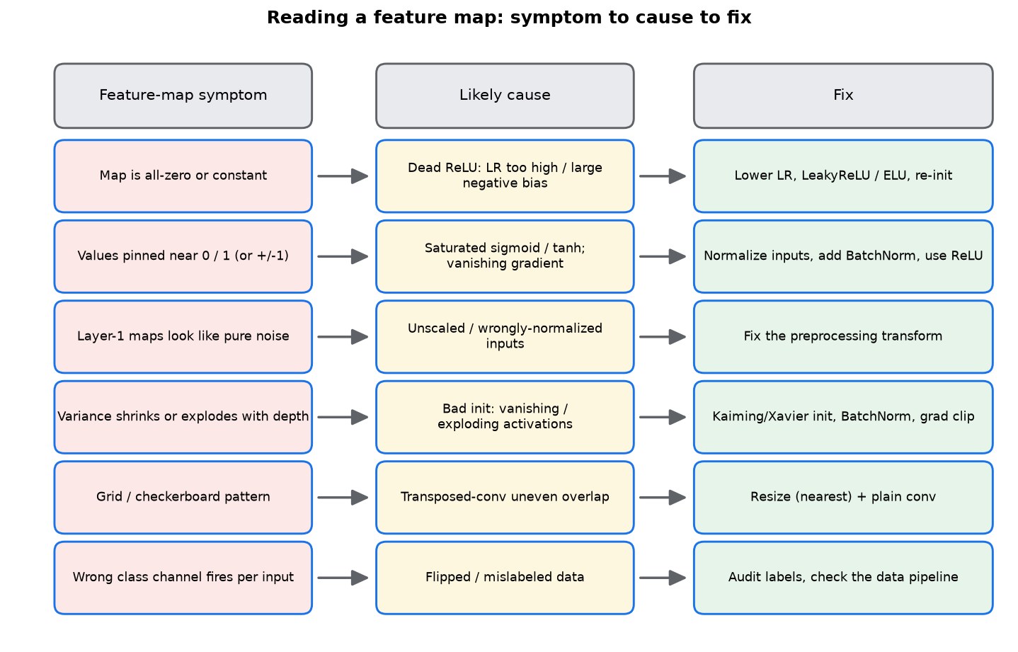
Put the pieces together and feature maps stop being a curiosity and become a routine. Feed a single batch, read the maps layer by layer, and match what you see to a cause and a fix — the loop in Fig 10.
The four tools that produce these views each have a sweet spot:
| Tool | What it shows | Reach for it when |
|---|---|---|
| register_forward_hook | Any layer's raw activations | Inspecting maps without editing the model |
| Matplotlib[4] / NumPy[12] | Channel grids, histograms, bars | Ad-hoc, one-batch inspection |
| TensorBoard[13] | Maps & histograms logged over training | Watching activations evolve across epochs |
| grad_cam | Pixels that drove a class | Explaining a specific prediction |
Key takeaways
- A forward hook (register_forward_hook) reads any layer's output without touching the model — the one primitive behind every figure here.
- Always establish the healthy look first: layer‑1 edge/stroke detectors deepening into part detectors. Every diagnosis is a comparison against it.
- Blank maps ⇒ dying ReLU (lower the LR, LeakyReLU/ELU); flat, pinned maps ⇒ saturation (normalize, batch-norm, re-init).
- Per-layer histograms catch vanishing/exploding activations early — watch the spread shrink or grow with depth.
- Noisy first-layer maps and 100×-too-large activations point at the data pipeline, not the model; a localized, symmetric confusion matrix points at labels.
- Over-sparse activations on unseen data accompany an overfit train/val gap; a checkerboard grid means a transposed-conv decoder — switch to resize‑then‑conv.
- Grad-CAM adds the class-driven view: which pixels drove the decision, not just what a filter responds to.
The complete, runnable code — the configurable Small_CNN, the Activation_Recorder, the training loop, the visualizers and the autoencoder — lives in the companion repository under src/; start with python src/train.py. Full attribution for the dataset and every library is in the repository's RESOURCES.md.
Resources
Every dataset, library, and paper cited above — numbered in order of first appearance. The digit images are rendered directly from MNIST under the license noted below. Click any bracketed marker such as [1] in the text to jump to its entry here.
- [1] MNIST — LeCun, Cortes & Burges, handwritten-digit database; freely available for research (commonly cited as CC BY-SA 3.0). yann.lecun.com/exdb/mnist
- [2] PyTorch — Paszke et al., An Imperative Style, High-Performance Deep Learning Library, NeurIPS 2019; register_forward_hook is part of torch.nn.Module. pytorch.org
- [3] torchvision — MNIST dataset wrapper and transforms. github.com/pytorch/vision
- [4] Matplotlib — J. D. Hunter, Matplotlib: A 2D Graphics Environment, CiSE 2007. matplotlib.org
- [5] Batch Normalization — Ioffe & Szegedy, Accelerating Deep Network Training by Reducing Internal Covariate Shift, ICML 2015. arXiv:1502.03167
- [6] Leaky ReLU — Maas, Hannun & Ng, Rectifier Nonlinearities Improve Neural Network Acoustic Models, ICML 2013. stanford.edu
- [7] ELU — Clevert, Unterthiner & Hochreiter, Fast and Accurate Deep Network Learning by Exponential Linear Units, ICLR 2016. arXiv:1511.07289
- [8] Kaiming initialization — He, Zhang, Ren & Sun, Delving Deep into Rectifiers, ICCV 2015. arXiv:1502.01852
- [9] Xavier/Glorot initialization — Glorot & Bengio, Understanding the difficulty of training deep feedforward neural networks, AISTATS 2010. proceedings.mlr.press
- [10] Checkerboard artifacts — Odena, Dumoulin & Olah, Deconvolution and Checkerboard Artifacts, Distill 2016. distill.pub
- [11] Grad-CAM — Selvaraju et al., Visual Explanations from Deep Networks via Gradient-based Localization, ICCV 2017. arXiv:1610.02391
- [12] NumPy — Harris et al., Array Programming with NumPy, Nature 2020. numpy.org
- [13] TensorBoard — TensorFlow/PyTorch visualization toolkit (torch.utils.tensorboard). tensorflow.org/tensorboard