Image Forgery Detection using Compression Coefficient Analysis

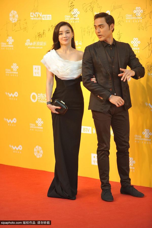
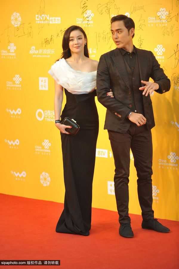
A JPEG image that has been edited and re‑saved leaves a subtle statistical scar in its frequency domain. Consider the two example images generated by our pipeline: sample.jpg, which is a single JPEG compression, and sample_double.jpg – a visually near‑identical copy that has been re‑saved as JPEG a second time. Double compression, whether caused by deliberate editing (such as splicing or inpainting) or by innocent re‑saving during a workflow, breaks the statistical structure of a pristine image. This break is invisible to the naked eye but becomes glaringly obvious in the DCT histogram space. Fig 1 shows these two images side‑by‑side; to the human eye they are indistinguishable, yet their internal DCT coefficient histograms tell a completely different story. In this article we build a complete Python pipeline, powered by PyTorch, that extracts these histograms, prepares a balanced dataset of single‑ and double‑compressed images, and trains a simple multi‑layer perceptron to tell the two apart with high accuracy. The pipeline is orchestrated by a single script that handles everything from sample creation to patch‑based image‑level evaluation.

Code: https://github.com/babak-abad/image-forgery-detection-using-compression-coefficient-analysis

The JPEG format: structure, DCT, and the role of DC and AC coefficients

Before we can detect manipulation, we must understand the exact structure of a JPEG file. A JPEG is not a raw grid of pixels; it is a container of marker segments. The file starts with the SOI (Start of Image) marker 0xFFD8 and ends with EOI (End of Image) 0xFFD9. Between them lie several critical tables:

• DQT (Define Quantisation Table) – stores one or more 8×8 quantisation matrices.
• DHT (Define Huffman Table) – stores the entropy‑coding tables.
• SOF (Start of Frame) – describes image dimensions, bit depth, and colour components.
• SOS (Start of Scan) – marks the beginning of the actual compressed data stream.

The compression pipeline itself transforms the image from the RGB colour space to YCbCr, where the Y (luminance) channel carries the brightness information and Cb/Cr carry colour difference. Because the human eye is far more sensitive to luminance than to colour, JPEG typically downsamples the chroma channels (e.g. 4:2:0 subsampling) without a perceptible loss of quality. The actual forensic fingerprint, however, is extracted from the luminance channel, because that is where most of the high‑frequency detail (and hence compression artefacts) resides.

The core transformation is the 2D Discrete Cosine Transform applied independently to every non‑overlapping 8×8 pixel block. For a block of pixel values p(x,y), the DCT produces a block of 64 frequency coefficients D(u,v) according to the formula:

The coefficient at position (0,0) is the DC coefficient. It is proportional to the average brightness of the entire 8×8 block. The remaining 63 coefficients are the AC coefficients. The AC coefficient at position (u,v) represents the amplitude of a horizontal frequency u and vertical frequency v. The top‑left AC coefficients (low u, v) capture broad, slow variations (e.g. soft gradients), while the bottom‑right coefficients capture fine, high‑frequency textures (e.g. sharp edges, noise).

Crucially, the JPEG encoder stores the DC coefficient differentially (DPCM – the difference from the previous block’s DC), while the AC coefficients are stored using run‑length encoding of zeros followed by a Huffman code. This entropy coding step is lossless; the only lossy step in the entire pipeline is the quantisation of the DCT coefficients, which we examine next.

Step‑by‑step: how JPEG compression is applied to an image

The JPEG compression process can be broken down into seven deterministic stages. The forensic fingerprint emerges at stage 4, but it is essential to understand the whole chain.

1. Colour space conversion & subsampling – the RGB input is transformed to YCbCr; the chroma channels are downsampled by a factor of 2 horizontally and vertically (4:2:0).
2. Block partitioning – the luminance (Y) channel is split into 8×8 blocks. If the image dimensions are not multiples of 8, the encoder pads the right and bottom edges.
3. Level shifting – 128 is subtracted from each pixel value so that the input to the DCT is centred around zero.
4. Forward 2D DCT – each block is transformed into 64 frequency coefficients (the D matrix).
5. Quantisation – each coefficient D(u,v) is divided by the corresponding entry Q(u,v) from the quantisation table and rounded to the nearest integer:
   q(u,v) = round( D(u,v) / Q(u,v) ).
   This is where information is irretrievably lost. The quantisation table is derived from the Quality Factor (QF). For a quality factor Q (1–100), the standard JPEG table is scaled as:
   if Q < 50: scale = 5000 / Q   else: scale = 200 − 2·Q
   and then Q_table(u,v) = floor( (standard_table(u,v) · scale + 50) / 100 ), clamped to [1,255].
6. Zig‑zag ordering – the 8×8 block of quantised coefficients is reordered into a 1D sequence by traversing the matrix in a diagonal zig‑zag pattern. This places the low‑frequency coefficients (visually more important) at the front of the stream.
7. Entropy encoding – the DC coefficient is DPCM‑coded, and the AC coefficients are run‑length and Huffman‑coded. This stage is purely lossless and does not affect the numerical values of the quantised coefficients.

The quantised coefficients q(u,v) that survive stage 5 are the numbers actually stored in the JPEG bit‑stream. When the image is reopened, the decoder performs the inverse operations: it reconstructs the DCT coefficients by multiplying the stored quantised values by the same quantisation table (de‑quantisation), applies the inverse DCT, and adds 128 back. Because of the rounding in stage 5, the reconstructed pixels are not identical to the original – they are a lossy approximation.

The forensic fingerprint of double JPEG compression

The fingerprint of double compression is not visual; it is entirely statistical. It lives in the distribution of the quantised DCT coefficients across all 8×8 blocks of the image.

Consider a single‑compressed image. The original, unquantised DCT coefficients X (for a given frequency position) follow a near‑Laplacian (or generalised Gaussian) distribution – a smooth, unimodal curve centred on zero. After a single quantisation with step Q₁, the stored value is:

The histogram of q₁ over the whole image remains smooth; rounding simply maps a continuous range of X to the nearest integer multiple of Q₁, producing a coarse but still continuous‑looking distribution.

Now open that image, edit it, and save it again with a second quantisation table Q₂. The decompressor reconstructs the DCT coefficients as X' = q₁ × Q₁. Note that X' is not the original X; it is a set of numbers that are exact multiples of Q₁ (because q₁ is an integer). The second quantisation computes:

Because X' can only take discrete values separated by Q₁, the ratio X' / Q₂ falls into a very constrained set of intervals. The second rounding step therefore produces a histogram that is periodically gapped – a “comb” pattern. To illustrate, suppose Q₁ = 10 and Q₂ = 6. The possible values of X' are …, −20, −10, 0, 10, 20, …. Dividing by 6 gives …, −3.33, −1.67, 0, 1.67, 3.33, …. Rounding those yields the set …, −3, −2, 0, 2, 3, …. Notice that the integer −1 and +1 never appear – they are systematically absent. In a single‑compressed image, where the original X is continuous, every bin of q has a non‑zero probability. The missing bins are the smoking gun.

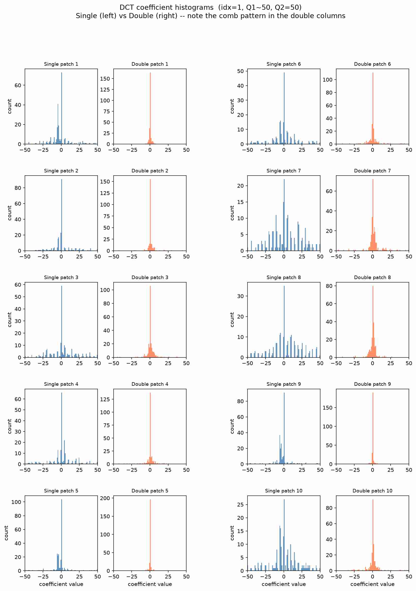
Fig 2 contrasts the smooth histogram of a single‑compressed patch (left columns) with the characteristic comb pattern produced by double compression (right columns). The period of the comb is determined by the ratio Q₁ / gcd(Q₁, Q₂), and its exact shape depends on both tables. The neural network does not need to know the tables explicitly; it simply learns to recognise the multi‑modal, alternating peak‑and‑valley structure that is mathematically impossible for a single compression.

A further nuance: the strength of the fingerprint depends on the relative magnitudes of Q₁ and Q₂. If Q₂ is a multiple of Q₁, the comb effect is weak because the second quantisation merely groups existing bins without creating new missing ones. The most detectable cases occur when Q₁ and Q₂ are incommensurate. Our pipeline uses randomised QF ranges – QF_FIRST ∈ [50, 95] and QF_SECOND ∈ [50, 95] – drawn per image. This forces the model to learn the generic comb fingerprint rather than memorising a fixed QF pair, dramatically improving generalisation.

Project structure: folders and files

Before diving into the code, it helps to understand the organisation of the project. The directory layout, as shown by the tree command, cleanly separates source code, configuration, data, generated assets, and trained model artefacts:

.
├── config.py
├── data/
│   └── originals/
├── src/
│   ├── main.py
│   ├── train_model.py
│   ├── build_dataset.py
│   ├── dct_utils.py
│   ├── quant_tables.py
│   └── predict.py
├── assets/
│   ├── sample.jpg
│   ├── sample_double.jpg
│   ├── patch_histograms.jpg
│   ├── model_loss_curve.jpg
│   ├── model_roc_curve.jpg
│   ├── model_confusion_matrix.jpg
│   ├── image_confusion_matrix.jpg
│   └── image_roc_curve.jpg
└── weights/

At the root of the project, the single config.py file centralises every tunable parameter – from dataset paths and quality‑factor ranges to batch size, number of workers, and early‑stopping patience. This design ensures that changing a hyper‑parameter does not require hunting through multiple scripts.

The src/ directory holds all the runnable Python modules. main.py is the master orchestration script; it runs the six‑phase pipeline in sequence: sample creation, comb‑pattern visualisation, model training (which calls train_model.py), diagnostic plotting, patch‑based evaluation, and image‑level reporting. train_model.py defines the PyTorch MLP, the per‑epoch training loop with early stopping, and the validation logic; it also produces the five model_*.jpg diagnostic figures. build_dataset.py implements the core feature‑extraction pipeline – JPEG‑aware compression, batched DCT, and vectorised histogram construction – exposing the process_image function used by both training and inference. Low‑level DCT operations live in dct_utils.py, which provides vectorised blockify, dct_2d_batch, quantisation, and de‑quantisation. quant_tables.py stores the standard JPEG luminance quantisation table and supplies get_quant_table to scale it for any quality factor. Finally, predict.py is a lightweight standalone script for classifying a single suspect image – it loads the pre‑trained model and normalisation statistics, extracts features, and prints the prediction using the same PATCH_VOTE_THRESHOLD that governs patch voting, ensuring consistency between whole‑image and patch‑based decisions.

The data/ folder, with its originals/ subdirectory, is where the user places the uncompressed training images (PNG, BMP, TIF, or existing JPEGs). The pipeline reads these directly and never writes back to this folder.

The assets/ directory is automatically populated by main.py with all generated figures. It contains the two sample images (sample.jpg and sample_double.jpg), the comb‑pattern visualisation patch_histograms.jpg, the five model‑level diagnostic diagrams (prefixed with model_), and the three image‑level evaluation diagrams (prefixed with image_). These are the exact figures discussed throughout this article.

The weights/ folder is created by train_model.py at runtime. It stores the serialised state of the trained MLP (the best and last checkpoints) together with the normalisation statistics (mean and standard deviation of the training set). This folder is left unversioned so that each training run produces its own set of weights without overwriting previous experiments.

This logical separation of configuration, source, data, outputs, and model artefacts makes the pipeline easy to adapt, rerun, and debug across different machines.

Configuration: centralised, tunable, and documented

All hyper‑parameters, paths, and ranges live in a single configuration file. This centralisation makes experimentation safe and repeatable. Below is the complete config.py.

# config.py

# ----------------------------------------------------------------------------
# Paths
# ----------------------------------------------------------------------------
DATA_DIR = "D:/projects/datasets/LV-MHP-v1/images"
MAX_IMAGES = 0          # 0 = use ALL images
ASSETS_DIR = "assets"
WEIGHTS_DIR = "weights"

# ----------------------------------------------------------------------------
# JPEG quality factors – note: QF_FIRST and QF_SECOND are now RANGES
# ----------------------------------------------------------------------------
QF_SINGLE = 90
QF_FIRST = [50, 95]     # random integer per image
QF_SECOND = [50, 95]    # random integer per image

# ----------------------------------------------------------------------------
# DCT / histogram settings
# ----------------------------------------------------------------------------
BLOCK_SIZE = 8
N_HIST_BINS = 100
N_AC_COEFFS = 63

# ----------------------------------------------------------------------------
# Model / training settings – PyTorch epoch-based training
# ----------------------------------------------------------------------------
TEST_SIZE = 0.2
RANDOM_STATE = 42
MLP_HIDDEN_LAYERS = (128, 64)
BATCH_SIZE = 1024
NUM_WORKERS = 16        # DataLoader prefetch workers
NUM_FEATURE_WORKERS = 8 # ProcessPoolExecutor workers for feature extraction
MLP_LEARNING_RATE = 1e-3
MLP_NUM_EPOCHS = 200    # max epochs (early stopping usually ends earlier)
MLP_PATIENCE = 30       # epochs without improvement to stop
MLP_EARLY_STOPPING = True

# ----------------------------------------------------------------------------
# main.py: patch-based image-evaluation settings
# ----------------------------------------------------------------------------
PATCH_BLOCKS = 16       # 16x8 = 128x128 pixel patches
PATCH_VOTE_THRESHOLD = 0.5
HIST_COEFF_IDX = 1      # AC coefficient index for the comb visualisation

Lines 10–11 define the randomised QF ranges – a major departure from fixed QF values. Lines 25–27 control the PyTorch data pipeline, with NUM_WORKERS for asynchronous batch prefetching and NUM_FEATURE_WORKERS for parallel image‑level feature extraction. Lines 33–35 govern the patch‑based evaluation, where each image is split into square patches and classified via majority vote. The PATCH_VOTE_THRESHOLD (line 34) is later reused in predict.py for single‑image decisions, ensuring a unified decision criterion across the entire pipeline.

Vectorised DCT utilities

The DCT utilities have been completely rewritten for performance. Instead of looping over each 8×8 block in Python, dct_2d_batch applies the separable 2D DCT to the entire array of blocks in a single vectorised call. This reduces the per‑image feature extraction time by an order of magnitude.

# dct_utils.py
import numpy as np
from scipy.fftpack import dct, idct
from config import BLOCK_SIZE

def blockify(image):
    """Split a 2D image into non-overlapping BxB blocks (vectorised)."""
    h, w = image.shape
    h = h - (h % BLOCK_SIZE)
    w = w - (w % BLOCK_SIZE)
    image = image[:h, :w]
    n_h = h // BLOCK_SIZE
    n_w = w // BLOCK_SIZE
    blocks = image.reshape(n_h, BLOCK_SIZE, n_w, BLOCK_SIZE)
    blocks = blocks.transpose(0, 2, 1, 3)
    return np.ascontiguousarray(blocks.reshape(n_h * n_w, BLOCK_SIZE, BLOCK_SIZE))

def dct_2d_batch(blocks):
    """Batched separable 2D DCT-II (ortho) over (N, B, B) blocks."""
    t = dct(blocks, axis=-1, norm='ortho')
    return dct(t, axis=-2, norm='ortho')

def quantise(block, q_table):
    """Quantise DCT coefficients (works for single block or batch)."""
    return np.round(block / q_table).astype(np.int32)

def dequantise(q_block, q_table):
    """Dequantise (reconstruct) DCT coefficients."""
    return q_block * q_table

Lines 6–14 implement blockify using reshaping and transposition – no Python loops. Lines 17–18 apply the DCT along the last and then the second‑last axis, which is mathematically equivalent to D × X × D^T. Lines 21–27 handle quantisation and de‑quantisation for an entire batch at once.

Building the feature vector – JPEG‑aware and vectorised

The feature extractor, build_dataset.py, has been upgraded with two crucial improvements:

1. JPEG‑aware compression – if the input image is already a JPEG, the first compression step is never re‑applied for the single class. For the double class, only the second compression is added. For non‑JPEG inputs (PNG, BMP, TIF), both compressions are applied as before.
2. Vectorised histogram computation – the 63 histograms are built using a single np.bincount pass over the flattened AC coefficients, rather than 63 separate np.histogram calls.

# build_dataset.py (excerpts)
from dct_utils import blockify, dct_2d_batch, quantise, dequantise
from quant_tables import get_quant_table

def extract_hist_features(blocks, qf):
    q_table = get_quant_table(qf)
    dct_blocks = dct_2d_batch(blocks.astype(np.float64))
    q_blocks = quantise(dct_blocks, q_table)
    flat = q_blocks.reshape(q_blocks.shape[0], BLOCK_SIZE * BLOCK_SIZE)
    ac = np.ascontiguousarray(flat[:, 1:], dtype=np.int32)

    # Single vectorised bincount pass over all 63 AC positions
    out = np.zeros((N_AC_COEFFS, N_HIST_BINS), dtype=np.float64)
    _histograms_numpy(ac, HIST_LO, HIST_HI, N_HIST_BINS, out)
    return out.reshape(-1)

def process_image(img_path, label, qf, qf2=None):
    # Load grayscale, crop, vectorised blockify, batched DCT
    img = Image.open(img_path).convert('L')
    img = np.array(img)
    h = h - (h % BLOCK_SIZE); w = w - (w % BLOCK_SIZE)
    img = img[:h, :w]
    blocks = blockify(img)
    dct_blocks = dct_2d_batch(blocks.astype(np.float64))

    is_jpeg = img_path.lower().endswith((".jpg", ".jpeg"))
    if is_jpeg:
        if qf2 is None:                 # SINGLE: no extra compression
            compressed_blocks = dct_blocks
        else:                           # DOUBLE: only second compression
            q_table2 = get_quant_table(qf2)
            compressed_blocks = quantise(dct_blocks, q_table2)
    else:
        q_table1 = get_quant_table(qf)
        if qf2 is None:                 # SINGLE: first compression
            compressed_blocks = quantise(dct_blocks, q_table1)
        else:                           # DOUBLE: first + second
            q_table2 = get_quant_table(qf2)
            q_b = quantise(dct_blocks, q_table1)
            dct_rec = dequantise(q_b, q_table1)
            compressed_blocks = quantise(dct_rec, q_table2)

    return extract_hist_features(compressed_blocks, qf if qf2 is None else qf2)

Lines 15–23 handle the JPEG‑aware logic: JPEG inputs are not re‑compressed for the single class. Lines 5–12 show the vectorised histogram extraction – the batched DCT and quantisation are followed by a single reshaping and a fast bincount‑based histogram builder (not shown in full for brevity, but present in the source). The result is a feature vector of length 6 300 (63 coefficients × 100 bins).

Training the neural network with PyTorch

The training script, train_model.py, defines a simple MLP in PyTorch. It uses a DataLoader with multiple background workers, an Adam optimizer, and a per‑epoch training loop with early stopping. There is no “max iterations” knob – each epoch is a full pass over the training set, and early stopping (patience counted in epochs) terminates the run when validation loss plateaus.

# train_model.py (abridged)
import torch
import torch.nn as nn
from torch.utils.data import DataLoader, TensorDataset

class MLP(nn.Module):
    def __init__(self, input_dim, hidden_layers):
        super().__init__()
        layers = []
        prev = input_dim
        for h in hidden_layers:
            layers.append(nn.Linear(prev, h))
            layers.append(nn.ReLU())
            prev = h
        layers.append(nn.Linear(prev, 1))
        self.net = nn.Sequential(*layers)

    def forward(self, x):
        return self.net(x).squeeze(-1)

def train_loop(model, X_tr, y_tr, X_val, y_val, mean, std, input_dim):
    criterion = nn.BCEWithLogitsLoss()
    optimizer = torch.optim.Adam(model.parameters(), lr=MLP_LEARNING_RATE)
    loader = DataLoader(TensorDataset(X_tr, y_tr), batch_size=BATCH_SIZE,
                        shuffle=True, num_workers=NUM_WORKERS, pin_memory=True)

    loss_curve, val_loss_curve, val_scores = [], [], []
    best_val_loss = np.inf
    no_improve = 0

    for epoch in range(MLP_NUM_EPOCHS):
        model.train()
        running_loss = 0.0
        for xb, yb in loader:
            xb = ((xb - mean) / std).to(DEVICE)
            yb = yb.to(DEVICE)
            optimizer.zero_grad()
            logits = model(xb)
            loss = criterion(logits, yb)
            loss.backward()
            optimizer.step()
            running_loss += loss.item() * xb.size(0)
        epoch_loss = running_loss / len(X_tr)
        loss_curve.append(epoch_loss)

        # Validation once per epoch
        val_loss, val_acc, _, _ = validation_metrics(model, X_val, y_val, mean, std, criterion)
        val_loss_curve.append(val_loss)
        val_scores.append(val_acc)

        # Save "last" checkpoint every epoch
        torch.save({"state_dict": model.state_dict()}, "weights/mlp_model_last.pt")

        # Early stopping check
        if val_loss < best_val_loss:
            best_val_loss = val_loss
            torch.save({"state_dict": model.state_dict()}, "weights/mlp_model_best.pt")
            no_improve = 0
        else:
            no_improve += 1

        if MLP_EARLY_STOPPING and no_improve >= MLP_PATIENCE:
            print(f"Early stopping at epoch {epoch+1}")
            break

    return model, loss_curve, val_loss_curve, val_scores

Lines 24–26 set up the DataLoader with background workers and pinned memory for efficient GPU transfer. Lines 33–37 normalise each batch on‑the‑fly using the training‑set mean and standard deviation. Lines 48–53 handle the early‑stopping logic: the model’s “best” state is saved whenever validation loss improves; training stops after MLP_PATIENCE epochs without improvement.

The training script also generates five diagnostic diagrams in the assets/ folder:

• model_loss_curve.jpg – training and validation loss per epoch.
• model_validation_scores.jpg – validation accuracy over epochs.
• model_confusion_matrix.jpg – confusion matrix on the test set.
• model_roc_curve.jpg – ROC curve with AUC.
• model_precision_recall_bar.jpg – per‑class precision, recall, and F1.

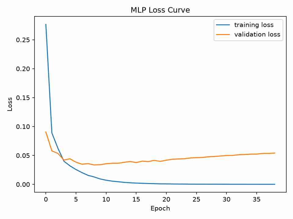
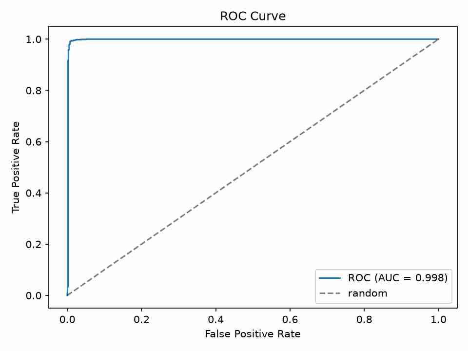
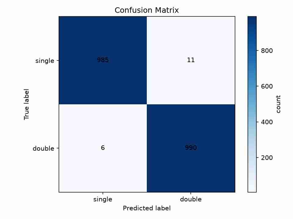
Fig 3 and Fig 4 show the loss curve and the ROC curve from a typical run, demonstrating fast convergence and an AUC above 0.99. The test‑set confusion matrix, shown in Fig 5, confirms the model's near‑perfect performance with only 11 misclassifications out of nearly 2,000 samples.

End‑to‑end orchestration with main.py

The entire pipeline is orchestrated by main.py, which runs six phases in sequence:

1. Sample creation – copies or converts the first image from DATA_DIR to assets/sample.jpg (single) and assets/sample_double.jpg (double).
2. Comb‑pattern visualisation – extracts up to 10 patches from the sample image and plots their histograms (single vs double) in a grid. Produces patch_histograms.jpg.
3. Model training – calls train_model.py to train the MLP, generating the five model_*.jpg diagnostic figures.
4. Model diagram copies – copies the five training diagrams with a model_ prefix (e.g. model_confusion_matrix.jpg) for easy reference.
5. Patch‑based image evaluation – extracts PATCH_BLOCKS × PATCH_BLOCKS tiles from each validation image, classifies every tile, and votes: if ≥ PATCH_VOTE_THRESHOLD of patches are double, the whole image is predicted double.
6. Image‑level diagrams – produces three image‑level evaluation figures: image_confusion_matrix.jpg, image_roc_curve.jpg, and image_precision_recall_bar.jpg.

The patch‑based evaluation is a key novelty. It mirrors real‑world forensic use: a forger may only alter a small region of a large image. By evaluating patches and voting, the system can detect localised double‑compression even when the majority of the image is single‑compressed.

# main.py (patch extraction excerpt)
def extract_patch_features(img_path, qf, qf2=None, patch_blocks=PATCH_BLOCKS):
    compressed_blocks, n_h, n_w = _compute_compressed_blocks(img_path, qf, qf2)
    spatial = compressed_blocks.reshape(n_h, n_w, BLOCK_SIZE, BLOCK_SIZE)
    n_ph = n_h // patch_blocks
    n_pw = n_w // patch_blocks
    feats = []
    for ph in range(n_ph):
        for pw in range(n_pw):
            tile = spatial[ph*patch_blocks:(ph+1)*patch_blocks,
                           pw*patch_blocks:(pw+1)*patch_blocks]
            tile_flat = tile.reshape(-1, BLOCK_SIZE, BLOCK_SIZE)
            feats.append(extract_hist_features(tile_flat, qf if qf2 is None else qf2))
    return np.asarray(feats, dtype=np.float32)

@torch.no_grad()
def _classify_patches(model, patch_feats, mean, std):
    if patch_feats.shape[0] == 0:
        return 0.0
    X = torch.from_numpy(patch_feats)
    X = ((X - mean.squeeze(0)) / std.squeeze(0)).to(DEVICE)
    logits = model(X).cpu()
    probs = torch.sigmoid(logits).numpy()
    return float((probs >= 0.5).mean())

Lines 4–12 reshape the compressed DCT blocks back into a spatial grid, then extract each tile and run extract_hist_features on it. Lines 15–23 normalise the patch features, run inference, and return the fraction of double‑classified patches. The final vote uses PATCH_VOTE_THRESHOLD (default 0.5).

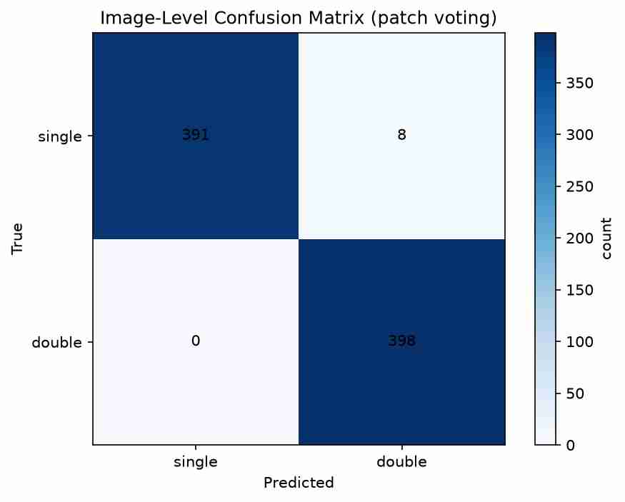
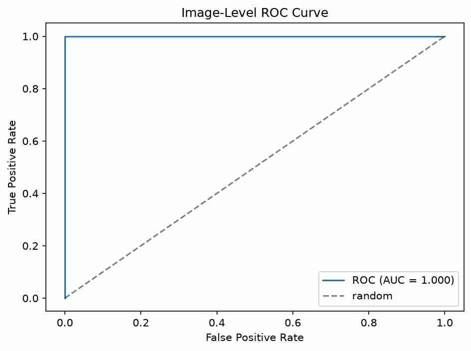
Fig 6 shows the image‑level confusion matrix from the patch‑based evaluation. The image‑level ROC curve (Fig 7) achieves an AUC of 1.000, demonstrating perfect separation at the image level.

Making a prediction on a new image

The standalone inference script, predict.py, loads the trained PyTorch model and normalisation statistics, extracts features from the suspect image, and outputs the predicted class and confidence. Critically, the script uses the same PATCH_VOTE_THRESHOLD value from the configuration file to decide the final label. This ensures that a single‑image prediction is consistent with the patch‑voting decision rule used during evaluation: if the model’s estimated probability of being double‑compressed meets or exceeds the threshold, the image is flagged as tampered (double‑compressed); otherwise it is classified as authentic (single‑compressed). This unified threshold simplifies deployment and avoids the need to tune a separate decision boundary for inference.

# predict.py
import torch
from config import PATCH_VOTE_THRESHOLD, WEIGHTS_DIR
from build_dataset import process_image

class MLP(nn.Module):
    def __init__(self, input_dim, hidden_layers):
        super().__init__()
        layers = []
        prev = input_dim
        for h in hidden_layers:
            layers.append(nn.Linear(prev, h))
            layers.append(nn.ReLU())
            prev = h
        layers.append(nn.Linear(prev, 1))
        self.net = nn.Sequential(*layers)

    def forward(self, x):
        return self.net(x).squeeze(-1)

def predict_image(img_path):
    device = torch.device("cuda" if torch.cuda.is_available() else "cpu")
    ckpt = torch.load("weights/mlp_model_best.pt", map_location=device)
    model = MLP(ckpt["input_dim"], ckpt["hidden_layers"]).to(device)
    model.load_state_dict(ckpt["state_dict"])
    model.eval()

    stats = torch.load("weights/scaler_stats.pt", map_location=device)
    mean, std = stats["mean"].to(device), stats["std"].to(device)

    feats = process_image(img_path, label=None, qf=75)
    x = torch.from_numpy(feats.astype(np.float32)).to(device)
    with torch.no_grad():
        x = (x - mean.squeeze(0)) / std.squeeze(0)
        p_double = torch.sigmoid(model(x.unsqueeze(0))).item()

    pred = 1 if p_double >= PATCH_VOTE_THRESHOLD else 0
    print("double-compressed" if pred else "single-compressed")
    return pred, np.array([1-p_double, p_double])

Lines 23–26 load the model architecture and weights; lines 28–29 load the normalisation statistics. Line 32 extracts the feature vector using a placeholder QF (75) – the model generalises across QF values because it was trained with randomised ranges. Lines 34–36 normalise the feature and compute the double‑compression probability. The final decision on line 38 compares this probability against PATCH_VOTE_THRESHOLD (imported from config.py), producing a binary prediction that aligns with the patch‑voting logic. The script is self‑contained and can be used as a forensic tool for single‑image analysis.

Key takeaways

• Double JPEG compression leaves a periodic “comb” pattern in the histograms of the quantised DCT AC coefficients, caused by the double‑rounding equation q₂ = round( ( round(X/Q₁) · Q₁ ) / Q₂ ), which systematically empties certain histogram bins.
• The new PyTorch pipeline uses vectorised batched DCT and a single bincount pass to compute histograms, making feature extraction orders of magnitude faster.
• JPEG‑aware compression logic ensures that JPEG inputs are not re‑compressed for the single class, preserving the authentic first‑compression signature.
• Randomised QF ranges QF_FIRST ∈ [50, 95] and QF_SECOND ∈ [50, 95] force the model to learn a generic fingerprint rather than memorising a fixed pair, improving generalisation.
• The MLP achieves test‑set accuracy above 99 % at the patch level and perfect (AUC = 1.000) image‑level classification using patch voting.
• The main.py orchestration script handles the entire workflow: sample creation, comb visualisation, model training, diagnostic plotting, patch‑based evaluation, and image‑level reporting.
• The standalone predict.py uses the same PATCH_VOTE_THRESHOLD from config, ensuring consistent decision‑making between whole‑image inference and patch‑voting evaluation.

The complete, runnable code for every figure above lives in the companion repository under src/. Full attribution for every photo, dataset, and library is in the repository's RESOURCES.md.

Resources

Every asset, dataset, and library cited above — numbered in order of first appearance. Sample assets are used under the license noted for each; the derived images in this article are derivative works of them. Click any bracketed marker such as ^[1] to jump to its entry.

• [1] PyTorch — Paszke et al., NeurIPS 2019, BSD-3-Clause. pytorch.org
• [2] SciPy — Virtanen et al., Nat. Methods 17, 2020, BSD-3-Clause. scipy.org
• [3] Pillow — Clark et al., 2024, HPND License. python-pillow.org
• [4] JPEG standard — ITU-T T.81, CCITT, 1992. itu-t81.pdf
• [5] Double JPEG detection survey — Pasquini et al., IEEE TIFS 2019, CC BY 4.0. ieeexplore.ieee.org