Deploying deep learning models on resource‑constrained devices demands a careful trade‑off between predictive performance and computational efficiency. Quantization – the process of reducing the numerical precision of weights and activations – is one of the most effective tools to achieve this balance. However, the practical implementation involves critical choices: post‑training quantization (PTQ) is quick and easy, while quantization‑aware training (QAT) often yields higher accuracy at the cost of additional training. In this comprehensive guide, we implement and benchmark eight different model quantization approaches on a simple CNN trained on Caltech‑101: FP32 (GPU), FP32 (CPU), FP16, BF16, PTQ‑Dynamic, PTQ‑Static, QAT, and a simulated 4‑bit method. We compare them on accuracy, precision, F1‑score, single‑image inference time, batch inference time, model size, and training time. Every line of code is dissected, and the entire project is organised as a clean, reusable repository with centralised configuration. The experimental results, obtained on an NVIDIA GPU with BF16 support, are presented and analysed in detail with seven comprehensive figures. Two separate runs are reported: the first run includes both GPU and CPU FP32 training, while the second run provides additional validation – the results are consistent and reproducible.
Code: https://github.com/babak-abad/Model-Quantization
Repository Structure and Full Code Walkthrough
The companion repository is organised as follows:
quantization-caltech101/
├── README.md
├── requirements.txt
├── config.py
├── src/
│   ├── __init__.py
│   ├── config.py
│   ├── data_loader.py
│   ├── evaluate.py
│   ├── model_utils.py
│   ├── model.py
│   ├── plotting.py
│   ├── ptq.py
│   ├── qat.py
│   ├── quant_4bit.py
│   ├── train.py
│   └── main.py
└── model_quantization_methods.md
Each file has a dedicated purpose:
- config.py – Centralised configuration (hyperparameters, paths, method flags).
- src/__init__.py – Empty, marks the folder as a package.
- data_loader.py – Downloads Caltech‑101, applies transformations, provides train/val/calibration loaders.
- evaluate.py – Evaluation metrics (accuracy, precision, F1) and inference timing with GPU synchronisation.
- model_utils.py – Saving/loading checkpoints, measuring file size.
- model.py – Defines the fusable CNN architecture with quantization stubs.
- plotting.py – Generates bar‑chart figures for all metrics with colour/hatch encoding.
- ptq.py – Post‑training static and dynamic quantization.
- qat.py – Quantization‑aware training from scratch.
- quant_4bit.py – Simulated 4‑bit weight quantization (research‑grade, with packed storage).
- train.py – Baseline FP32 training loop.
- main.py – Orchestrates the entire pipeline: training, all 8 methods, evaluation, timing, and figure generation.
Quantization Fundamentals
Quantization maps a floating‑point tensor x (usually FP32) to an integer tensor xq using a scale factor S and a zero‑point Z. For symmetric quantization, Z = 0 and S = max(|x|) / 127 (for signed INT8). Asymmetric quantization, often used for activations (which may be non‑negative after ReLU), employs S = (max(x) - min(x)) / 255 and Z = -min(x) / S (rounded to nearest integer). The mapping is:
xq = clamp( round( x / S + Z ), 0, 255 )
xapprox = S × ( xq - Z )
The clamp ensures the integer stays within range. The approximation errors stem from rounding and clipping. The choice of per‑tensor vs per‑channel scaling further affects accuracy. In our implementation, we use per‑tensor symmetric for weights and per‑tensor asymmetric for activations, which is the default for the fbgemm backend.
Why does quantization speed up inference? The primary source of speedup comes from integer arithmetic. Processors are optimised for low‑precision integer operations; a single 32‑bit floating‑point multiplication may take several cycles, while an 8‑bit integer multiply‑add can often be executed in a single cycle. Modern CPUs feature SIMD (Single Instruction, Multiple Data) extensions such as AVX‑512, which can process sixteen 8‑bit integers in parallel, delivering a theoretical throughput that is 4–8× higher than FP32. Furthermore, integer operations consume less energy – a critical factor for battery‑powered devices. The reduced bit width also cuts memory bandwidth requirements: a model that occupies 40 MB in FP32 shrinks to 10 MB in INT8. This lowers the latency of loading weights from DRAM into caches, and smaller tensors fit more comfortably in fast on‑chip caches, reducing cache misses. On specialised hardware like NVIDIA Tensor Cores, ARM Neon, or Google TPUs, integer computation is not only faster but can be further accelerated by dedicated systolic arrays that exploit the dense, regular nature of quantised matrix multiplications. In short, the speedup is a multiplicative gain from both arithmetic efficiency and improved memory hierarchy utilisation.
But why does quantization hurt accuracy? The approximation error introduced by quantization manifests in two main forms: rounding error and clipping error. Rounding error arises because the integer grid has finite granularity; values that fall between two discrete integer levels are rounded to the nearest one, effectively adding noise to the weights and activations. Clipping error occurs when values exceed the representable range (e.g., a weight larger than 127 * S is truncated to the maximum integer), which can discard important information, especially in the presence of outliers. This noise propagates through the network and alters the feature maps, potentially shifting decision boundaries. Moreover, the loss landscape of deep networks is highly non‑convex; a small perturbation in the weights can cause the output logits to deviate significantly, particularly for layers with large condition numbers. The effect is not uniform – certain layers are more sensitive to quantization than others. For example, the first convolutional layer often sees a wide dynamic range of pixel intensities, and fully‑connected layers near the classifier may be sensitive to small changes in their large‑magnitude weights. If we quantise without any adaptation, the model’s internal representations no longer align with the training distribution, leading to a drop in classification performance.
The role of outliers and calibration. Outliers in weight or activation distributions are particularly harmful in symmetric quantization because the scale factor is determined by the maximum absolute value – a single large outlier can dominate the scale, leaving most of the quantised range under‑utilised and wasting resolution. This is why per‑channel scaling (different scales for each output channel of a convolution) often outperforms per‑tensor scaling: it isolates the effect of outliers to the channel where they occur. In post‑training quantization, calibration (running a small subset of training data to collect activation statistics) is crucial because it determines the clipping range. If the calibration set is not representative, the observed min/max values will be skewed, and the model may clip many activations during inference, causing severe accuracy degradation. In practice, choosing a calibration set of 200–500 samples that mirrors the validation distribution is a delicate balancing act – too few samples and you miss important data points; too many and the calibration becomes slow. This is one reason why quantization‑aware training (QAT) is attractive: it learns the scale and zero‑point during training, adapting them to the real data distribution while also forcing the weights to adjust to the quantisation noise.
Why QAT recovers accuracy. QAT simulates quantization during the forward pass by inserting fake quant operations. This injects noise that resembles rounding and clipping, but crucially, the gradients are passed through using a straight‑through estimator – the loss is computed on the dequantised (but quantised‑approximated) outputs, and the gradients are backpropagated as if the quantiser were the identity function. This allows the model to learn weights that are robust to the quantization noise, essentially “folding” the error into the optimisation. The network finds a local minimum that lies in a region where the weights are not sensitive to small perturbations, and the scale factors are updated to optimally cover the activation ranges. As a result, QAT can often close the accuracy gap to within 1–2% of the FP32 baseline, as we will see in our experiments.
Trade‑off and practical considerations. The speedup is nearly free – once the model is quantised, the latency and memory improvements are automatic. The cost is the potential loss in accuracy and the additional engineering complexity (fusion, calibration, conversion). For many real‑world applications, an accuracy drop of 1–2% is perfectly acceptable given the 3–4× speedup and 4× memory reduction. However, for safety‑critical systems (e.g., medical imaging, autonomous driving), even small drops may be unacceptable, and QAT becomes a necessary investment. In the next sections, we will quantify these effects with a concrete implementation on Caltech‑101.
Method Overview
The following table summarises the eight methods benchmarked in this project. Each method is implemented in the corresponding module and evaluated on the same validation set.
| # | Method | Device | Precision | Weights | Activations | Needs Training? | Needs Calibration? |
|---|---|---|---|---|---|---|---|
| 1 | FP32 (GPU) | GPU | 32-bit float | FP32 | FP32 | ✅ from scratch | ❌ |
| 2 | FP32 (CPU) | CPU | 32-bit float | FP32 | FP32 | ✅ from scratch | ❌ |
| 3 | FP16 | GPU | 16-bit float | FP16 | FP16 | ❌ post-training | ❌ |
| 4 | BF16 | GPU | Bfloat16 | BF16 | BF16 | ❌ post-training | ❌ |
| 5 | PTQ-Dynamic | CPU | 8-bit int (weights only) | INT8 | FP32 (dynamic) | ❌ post-training | ❌ |
| 6 | PTQ-Static | CPU | 8-bit int | INT8 | INT8 | ❌ post-training | ✅ |
| 7 | QAT | CPU | 8-bit int | INT8 | INT8 | ✅ from scratch | ❌ |
| 8 | 4-bit Sim | CPU | 4-bit int (simulated) | INT4 | FP32 | ❌ post-training | ❌ |
Complete Code Walkthrough – Line‑by‑Line
We now provide a thorough, line‑by‑line explanation of every module in the src/ folder. Each code block is presented in full, followed by a detailed breakdown of every statement, function, and design choice. Where a file is long (e.g., main.py), we split it into logical sections to keep the explanations clear. The full source code is available in the companion repository; the explanations below cover every line.
File: config.py
This module is the single source of truth for all hyperparameters, paths, and method‑specific settings. It uses dataclasses to organise settings into logical groups, making the code maintainable and self‑documenting. Every other module imports the singleton config instance to access settings.
"""Centralized configuration for the Model-Quantization project.

All hard-coded values that were previously scattered across modules live here.
Import the singleton ``config`` instance anywhere you need a setting:

    from src.config import config
    print(config.hyperparams.epochs)
"""

import torch
import torch.nn as nn
from dataclasses import dataclass, field
from typing import List, Tuple, Set
Line 1: The opening triple‑quote begins the module docstring.
Lines 2–6: The docstring explains the purpose of centralising configuration and provides a usage example.
Line 8: Import torch – needed for device detection and BF16 support checks.
Line 9: Import torch.nn as nn – needed to define the set of layer types for dynamic quantization (e.g., nn.Linear).
Line 10: Import dataclass and field from the dataclasses module – these allow us to define clean, immutable configuration classes with default values and automatic __init__ methods.
Line 11: Import typing hints – List, Tuple, Set – for better code readability and to enable static type checking with tools like mypy.
# --------------------------------------------------------------------------- #
# Shared training / learning hyperparameters
# --------------------------------------------------------------------------- #
@dataclass
class TrainingHyperparameters:
    """Single source of truth for batch size and learning hyperparameters.

    These values are shared across every training stage (FP32 baseline, QAT)
    and evaluation so that the batch size, learning rate, schedule, etc. never
    drift out of sync between modules.
    """

    batch_size: int = 64
    epochs: int = 10
    lr: float = 1e-3
    scheduler_factor: float = 0.1
    scheduler_patience: int = 3
    grad_clip: float = 1.0
Line 13: A comment separator visually groups related settings.
Line 14: Another comment for clarity.
Line 15: The @dataclass decorator tells Python to generate an __init__ method, __repr__, and other methods automatically.
Line 16: class TrainingHyperparameters – defines the core hyperparameters used during training.
Lines 17–21: Docstring explaining that these values are shared across FP32 and QAT to ensure consistency.
Line 23: batch_size: int = 64 – the number of samples per batch. This is a common size that balances memory and convergence speed.
Line 24: epochs: int = 10 – the number of training passes over the entire dataset. We use 10 for this experiment to keep training fast.
Line 25: lr: float = 1e-3 – the initial learning rate for the Adam optimizer. This value works well for many computer vision tasks.
Line 26: scheduler_factor: float = 0.1 – the factor by which the learning rate is multiplied when the validation error plateaus. A factor of 0.1 reduces LR by 90% to help the model settle at a better minimum.
Line 27: scheduler_patience: int = 3 – the number of epochs without improvement before reducing LR. If the validation error does not decrease for 3 consecutive epochs, the scheduler triggers.
Line 28: grad_clip: float = 1.0 – the maximum gradient norm used to prevent exploding gradients. Clipping gradients at 1.0 is a safe default that helps stabilise training.
# --------------------------------------------------------------------------- #
# Data pipeline
# --------------------------------------------------------------------------- #
@dataclass
class DataConfig:
    data_dir: str = "./data"
    val_split: float = 0.2          # fraction of the dataset used for validation
    calib_samples: int = 200        # number of calibration images for PTQ
    calib_batch_size: int = 32
    # Windows + CUDA can BSOD when DataLoader spawns many worker processes.
    # Keep this at 0 unless you've confirmed stability on your machine.
    num_workers: int = 0
    pin_memory: bool = False          # auto-enabled for CUDA in get_dataloaders
    persistent_workers: bool = False  # only takes effect when num_workers > 0
    drop_last: bool = True            # drop irregular final batch (training)
    image_size: Tuple[int, int] = (128, 128)
    target_type: str = "category"
    download: bool = False
    # ImageNet normalization statistics (works well for transfer / general images)
    normalize_mean: Tuple[float, float, float] = (0.485, 0.456, 0.406)
    normalize_std: Tuple[float, float, float] = (0.229, 0.224, 0.225)
Line 30: Data pipeline section header.
Line 31: Another comment.
Line 32: @dataclass – decorator.
Line 33: class DataConfig – stores all dataset‑related configuration.
Line 34: data_dir: str = "./data" – the directory where the dataset will be downloaded and stored.
Line 35: val_split: float = 0.2 – reserves 20% of the dataset for validation. This is a typical split that gives enough data for training while providing a representative validation set.
Line 36: calib_samples: int = 200 – the number of images used for calibration in static PTQ. 200 samples are enough to estimate the activation ranges while keeping the calibration step fast.
Line 37: calib_batch_size: int = 32 – batch size during calibration. A smaller batch than training helps keep memory usage low.
Line 38: A comment warning about potential issues with Windows and CUDA when using multiple workers – this is a known PyTorch issue where setting num_workers > 0 can cause a blue screen of death (BSOD) on some Windows systems.
Line 39: Comment explaining the default value.
Line 40: num_workers: int = 0 – set to 0 to avoid multiprocessing issues. This means data loading will be done in the main process, which is safe but slightly slower.
Line 41: pin_memory: bool = False – auto‑enabled if CUDA is available in get_dataloaders. Pinned memory speeds up host‑to‑GPU transfers.
Line 42: persistent_workers: bool = False – only used if num_workers > 0. Persistent workers keep the worker processes alive between epochs, which can improve performance.
Line 43: drop_last: bool = True – drops the final incomplete batch during training. This keeps batch normalisation statistics consistent because all batches have the same size.
Line 44: image_size: Tuple[int, int] = (128, 128) – images are resized to 128×128 pixels. This resolution is a good trade‑off between computational cost and classification accuracy for a small CNN.
Line 45: target_type: str = "category" – specifies that we want category labels (integers) rather than image IDs.
Line 46: download: bool = False – if True, the dataset will be downloaded automatically. We set it to False by default because the user might already have the dataset; they can set it to True if needed.
Line 47: Comment explaining the normalisation statistics.
Line 48: normalize_mean: Tuple[float, float, float] = (0.485, 0.456, 0.406) – mean values for each RGB channel, derived from ImageNet. These are commonly used for transfer learning.
Line 49: normalize_std: Tuple[float, float, float] = (0.229, 0.224, 0.225) – standard deviations for each RGB channel, also from ImageNet.
# --------------------------------------------------------------------------- #
# Model architecture
# --------------------------------------------------------------------------- #
@dataclass
class ModelConfig:
    num_classes: int = 101
    input_channels: int = 3
    conv_channels: List[int] = field(default_factory=lambda: [32, 64, 128])
    fc_hidden: int = 256
    kernel_size: int = 3
    padding: int = 1
    # (conv → relu → maxpool) pairs, each pool halves spatial dims
    num_pool_layers: int = 3
    # Module groups to fuse during quantization
    fuse_modules: List[List[str]] = field(
        default_factory=lambda: [
            ["conv1", "relu1"],
            ["conv2", "relu2"],
            ["conv3", "relu3"],
            ["fc1", "relu4"],
        ]
    )

    def flattened_size(self, image_size: Tuple[int, int]) -> int:
        """Compute the flattened feature-map size after all conv/pool layers."""
        out_channels = self.conv_channels[-1]
        spatial = image_size[0] // (2 ** self.num_pool_layers)
        return out_channels * spatial * spatial
Line 51: Model architecture section header.
Line 52: Comment.
Line 53: @dataclass.
Line 54: class ModelConfig – defines the CNN structure.
Line 55: num_classes: int = 101 – Caltech‑101 has 101 object categories plus a background class, so the total is 101 (the background is included in the dataset’s categories list). We set this to 101.
Line 56: input_channels: int = 3 – RGB images have 3 channels.
Line 57: conv_channels: List[int] = field(default_factory=lambda: [32, 64, 128]) – a list of the number of filters in each of the three convolutional layers. The lambda creates a new list each time the dataclass is instantiated, preventing shared mutable state.
Line 58: fc_hidden: int = 256 – the size of the first fully‑connected layer. This is a common hidden size for small CNNs.
Line 59: kernel_size: int = 3 – the convolution kernel size. 3×3 kernels are standard and capture local features well.
Line 60: padding: int = 1 – padding of 1 ensures the spatial size is preserved (same convolution).
Line 61: Comment about pooling layers.
Line 62: num_pool_layers: int = 3 – three max‑pooling layers, each halving the spatial size. Starting from 128×128, after three pools we get 16×16.
Line 63: Comment about fusion.
Lines 64–70: fuse_modules: List[List[str]] = field(...) – a list of module name pairs for fusion during quantization. Each inner list pairs a convolution with its ReLU, and the first FC layer with its ReLU. This is required for PyTorch’s fuse_modules.
Line 72: def flattened_size(self, image_size: Tuple[int, int]) -> int: – a method that computes the input size to the first linear layer.
Line 73: Docstring.
Line 74: out_channels = self.conv_channels[-1] – the number of output channels from the last convolution (128).
Line 75: spatial = image_size[0] // (2 ** self.num_pool_layers) – divide the image width by 2 raised to the number of pooling layers. For 128 and 3 pools, this gives 128 // 8 = 16.
Line 76: return out_channels * spatial * spatial – multiply to get the total number of features (128 * 16 * 16 = 32,768).
The remaining config classes (TrainConfig, PTQConfig, QATConfig, Float16Config, Quant4BitConfig, EvalConfig, PathConfig, PlotConfig, and the aggregate Config) are included in the full source code. They follow the same pattern: each dataclass groups related settings, and the Config class composes them all. The get_device method returns CUDA if available, get_quant_device always returns CPU (because fbgemm int8 kernels are CPU‑only), and bf16_supported checks for Ampere+ architecture by inspecting the compute capability.
File: data_loader.py
This module is responsible for downloading the Caltech‑101 dataset, applying necessary image transformations, and creating the three data loaders used throughout the experiment: training, validation, and calibration. The calibration loader is a small subset of the training set used exclusively for static PTQ.
import torch
from torchvision import datasets, transforms
from torch.utils.data import DataLoader, random_split, Subset

try:
    from src.config import config
except ImportError:
    from config import config


class _ConvertToRGB:
    """Picklable transform that converts images to RGB (handles grayscale images)."""
    def __call__(self, img):
        return img.convert('RGB')
Line 1: Import torch – needed for CUDA availability checks.
Line 2: Import datasets and transforms from torchvision. datasets.Caltech101 provides the dataset class; transforms contains image preprocessing utilities.
Line 3: Import DataLoader, random_split, and Subset from torch.utils.data. DataLoader handles batching and shuffling; random_split partitions the dataset; Subset is used to create the calibration subset.
Lines 5–8: Try to import config from src.config. If that fails (e.g., when running the script standalone), fall back to a local config import. This makes the module flexible for both package and standalone use.
Line 11: Define _ConvertToRGB class. It is a callable class, so it can be used as a transform. The docstring explains that it converts images to RGB and is picklable (important for multiprocessing).
Line 12: The __call__ method makes the class callable.
Line 13: return img.convert('RGB') – converts the PIL image to RGB. This handles grayscale images, which occasionally appear in Caltech‑101, by converting them to three‑channel RGB.
def get_dataloaders(data_dir=None, batch_size=None, val_split=None,
                    calib_samples=None, num_workers=None):
    dc = config.data
    hp = config.hyperparams
    data_dir = dc.data_dir if data_dir is None else data_dir
    batch_size = hp.batch_size if batch_size is None else batch_size
    val_split = dc.val_split if val_split is None else val_split
    calib_samples = dc.calib_samples if calib_samples is None else calib_samples
    num_workers = dc.num_workers if num_workers is None else num_workers

    transform = transforms.Compose([
        _ConvertToRGB(),
        transforms.Resize(dc.image_size),
        transforms.ToTensor(),
        transforms.Normalize(mean=dc.normalize_mean, std=dc.normalize_std)
    ])
Line 15: Function signature – takes optional overrides for data_dir, batch_size, val_split, calib_samples, and num_workers. If not provided, it uses the values from config.
Line 17: dc = config.data – alias for the data config.
Line 18: hp = config.hyperparams – alias for hyperparameters.
Lines 19–23: Assign local variables. The if ... is None pattern allows function arguments to override config values. If an argument is None, we use the config value.
Lines 25–30: Build the transformation pipeline using transforms.Compose. The pipeline consists of:
- _ConvertToRGB() – ensures images are RGB.
- transforms.Resize(dc.image_size) – resizes to 128×128.
- transforms.ToTensor() – converts to a PyTorch tensor and scales pixel values to [0,1].
- transforms.Normalize(mean=dc.normalize_mean, std=dc.normalize_std) – normalises using ImageNet statistics. This helps with convergence because the input features are centered around zero.
    full_dataset = datasets.Caltech101(
        root=data_dir, target_type=dc.target_type,
        transform=transform, download=dc.download
    )
    num_classes = len(full_dataset.categories)
    val_size = int(val_split * len(full_dataset))
    train_size = len(full_dataset) - val_size
    train_dataset, val_dataset = random_split(full_dataset, [train_size, val_size])

    # Auto-enable pin_memory on CUDA for faster host→GPU copies.
    use_pin_memory = dc.pin_memory and torch.cuda.is_available()
    # persistent_workers is only valid when num_workers > 0.
    use_persistent = dc.persistent_workers and num_workers > 0
Line 32: full_dataset = datasets.Caltech101(...) – loads the Caltech‑101 dataset. It uses the provided data_dir as the root, target_type (category), the transformation pipeline, and download flag. If the dataset is not already present and download is True, it will be downloaded.
Line 36: num_classes = len(full_dataset.categories) – the number of categories in the dataset. This is used to set the model’s output size.
Line 37: val_size = int(val_split * len(full_dataset)) – compute the number of validation samples based on the split ratio.
Line 38: train_size = len(full_dataset) - val_size – the rest is training.
Line 39: train_dataset, val_dataset = random_split(full_dataset, [train_size, val_size]) – randomly splits the dataset into training and validation subsets. This preserves the class distribution approximately because the split is random.
Line 42: use_pin_memory = dc.pin_memory and torch.cuda.is_available() – if pin_memory is True and CUDA is available, we enable pinned memory. Pinned memory is faster for CPU‑to‑GPU transfers because the memory is page‑locked.
Line 44: use_persistent = dc.persistent_workers and num_workers > 0 – only enable persistent workers if persistent_workers is True and num_workers > 0. Persistent workers keep worker processes alive across epochs, which can reduce overhead.
    train_loader = DataLoader(
        train_dataset, batch_size=batch_size, shuffle=True,
        num_workers=num_workers, pin_memory=use_pin_memory,
        persistent_workers=use_persistent, drop_last=dc.drop_last,
    )
    val_loader = DataLoader(
        val_dataset, batch_size=batch_size, shuffle=False,
        num_workers=num_workers, pin_memory=use_pin_memory,
        persistent_workers=use_persistent,
    )
    calib_subset = Subset(train_dataset, range(min(calib_samples, len(train_dataset))))
    calib_loader = DataLoader(
        calib_subset, batch_size=dc.calib_batch_size, shuffle=False,
        num_workers=0,  # calibration is short — no need for worker processes
    )
    return train_loader, val_loader, calib_loader, num_classes
Line 46: train_loader = DataLoader(...) – creates the training loader. It uses the training dataset, the specified batch size, shuffles the data, and uses the configured num_workers, pin_memory, persistent_workers, and drop_last. Shuffling is essential for training to prevent the model from learning batch order.
Line 50: The drop_last=True ensures that the final incomplete batch is dropped so that all batches have the same size, which is important for batch normalisation.
Line 52: val_loader – similar to the training loader but with shuffle=False because we want deterministic evaluation.
Line 57: calib_subset = Subset(train_dataset, range(min(calib_samples, len(train_dataset)))) – creates a subset of the training dataset using the first calib_samples samples. The min ensures we don’t exceed the dataset size.
Line 58: calib_loader = DataLoader(...) – calibration loader with calib_batch_size, no shuffling, and num_workers=0 because calibration is short and we avoid the overhead of parallel workers.
Line 61: Return the three loaders and the number of classes.
File: model.py
Defines the Fusable_Simple_CNN with quantization stubs.
import torch.nn as nn
from torch.quantization import QuantStub, DeQuantStub

try:
    from src.config import config
except ImportError:
    from config import config


class Fusable_Simple_CNN(nn.Module):
    def __init__(self, num_classes=None):
        super().__init__()
        mc = config.model
        if num_classes is None:
            num_classes = mc.num_classes

        ch = mc.conv_channels          # e.g. [32, 64, 128]
        in_c = mc.input_channels       # 3
        k, p = mc.kernel_size, mc.padding

        self.quant = QuantStub()
        self.conv1 = nn.Conv2d(in_c, ch[0], kernel_size=k, padding=p)
        self.relu1 = nn.ReLU()
        self.pool1 = nn.MaxPool2d(2, 2)
        self.conv2 = nn.Conv2d(ch[0], ch[1], kernel_size=k, padding=p)
        self.relu2 = nn.ReLU()
        self.pool2 = nn.MaxPool2d(2, 2)
        self.conv3 = nn.Conv2d(ch[1], ch[2], kernel_size=k, padding=p)
        self.relu3 = nn.ReLU()
        self.pool3 = nn.MaxPool2d(2, 2)
        self.fc1 = nn.Linear(mc.flattened_size(config.data.image_size), mc.fc_hidden)
        self.relu4 = nn.ReLU()
        self.fc2 = nn.Linear(mc.fc_hidden, num_classes)
        self.dequant = DeQuantStub()

    def forward(self, x):
        x = self.quant(x)
        x = self.pool1(self.relu1(self.conv1(x)))
        x = self.pool2(self.relu2(self.conv2(x)))
        x = self.pool3(self.relu3(self.conv3(x)))
        x = x.reshape(x.size(0), -1)
        x = self.relu4(self.fc1(x))
        x = self.fc2(x)
        x = self.dequant(x)
        return x
Line 1: Import torch.nn as nn – provides layers like Conv2d, ReLU, MaxPool2d, Linear.
Line 2: Import QuantStub and DeQuantStub from torch.quantization. These are placeholder modules that will be replaced during quantization preparation.
Lines 4–7: Import config with fallback.
Line 10: class Fusable_Simple_CNN(nn.Module) – inherits from PyTorch’s base module class.
Line 11: Constructor – takes optional num_classes. If not provided, reads from config.model.num_classes.
Line 12: super().__init__() – calls the parent class constructor.
Line 13: mc = config.model – alias for model config.
Lines 14–15: If num_classes is None, use the config value.
Lines 17–19: Extract channel sizes, input channels, kernel size, and padding from mc.
Line 21: self.quant = QuantStub() – a placeholder that marks the input boundary for quantization. During prepare or prepare_qat, this will be replaced by a FakeQuantize module (in QAT) or a real quantizer (in PTQ).
Line 22: self.conv1 = nn.Conv2d(in_c, ch[0], kernel_size=k, padding=p) – first convolutional layer. Takes 3 input channels, outputs 32 channels, uses 3×3 kernel and padding=1 to preserve spatial size.
Line 23: self.relu1 = nn.ReLU() – ReLU activation after conv1. Stored separately for fusion.
Line 24: self.pool1 = nn.MaxPool2d(2, 2) – 2×2 max‑pooling reduces spatial size by half.
Line 25: self.conv2 = nn.Conv2d(ch[0], ch[1], kernel_size=k, padding=p) – second convolution: 32 → 64 channels.
Line 26: self.relu2 = nn.ReLU() – ReLU for conv2.
Line 27: self.pool2 = nn.MaxPool2d(2, 2) – second pooling.
Line 28: self.conv3 = nn.Conv2d(ch[1], ch[2], kernel_size=k, padding=p) – third convolution: 64 → 128 channels.
Line 29: self.relu3 = nn.ReLU() – ReLU for conv3.
Line 30: self.pool3 = nn.MaxPool2d(2, 2) – third pooling.
Line 31: self.fc1 = nn.Linear(mc.flattened_size(config.data.image_size), mc.fc_hidden) – the first fully‑connected layer. Its input size is computed by mc.flattened_size(), which uses the image size and number of pooling layers. The output is 256 (hidden size).
Line 32: self.relu4 = nn.ReLU() – ReLU after fc1. Stored separately for fusion.
Line 33: self.fc2 = nn.Linear(mc.fc_hidden, num_classes) – final linear layer mapping to the number of classes.
Line 34: self.dequant = DeQuantStub() – placeholder for output dequantisation.
Line 37: def forward(self, x): – defines the forward pass.
Line 38: x = self.quant(x) – applies the quant stub (quantises input in quantized mode).
Line 39: x = self.pool1(self.relu1(self.conv1(x))) – applies conv1, ReLU, and pool1.
Line 40: x = self.pool2(self.relu2(self.conv2(x))) – conv2, ReLU, pool2.
Line 41: x = self.pool3(self.relu3(self.conv3(x))) – conv3, ReLU, pool3.
Line 42: x = x.reshape(x.size(0), -1) – flattens the tensor. x.size(0) is the batch size, -1 infers the remaining dimensions.
Line 43: x = self.relu4(self.fc1(x)) – applies fc1 and ReLU.
Line 44: x = self.fc2(x) – final linear layer.
Line 45: x = self.dequant(x) – dequantises the output (if quantized mode, returns FP32).
Line 46: return x – returns the logits.
File: train.py
Contains the baseline FP32 training loop with Adam, LR scheduler, and checkpoint saving. The same function is used for both GPU and CPU training (device is passed as an argument).
import torch
import torch.nn as nn
import torch.optim as optim
from torch.optim.lr_scheduler import ReduceLROnPlateau

try:
    from src.config import config
    from src.evaluate import evaluate
    from src.model_utils import save_model
except ImportError:
    from config import config
    from evaluate import evaluate
    from model_utils import save_model


def train_baseline(model, train_loader, val_loader, epochs=None, lr=None, device=None):
    tc = config.train
    hp = config.hyperparams
    epochs = hp.epochs if epochs is None else epochs
    lr = hp.lr if lr is None else lr
    if device is None:
        device = config.get_device()
    model.to(device)
    criterion = nn.CrossEntropyLoss()
    optimizer = optim.Adam(model.parameters(), lr=lr)
    scheduler = ReduceLROnPlateau(
        optimizer, mode='min', factor=hp.scheduler_factor, patience=hp.scheduler_patience
    )

    best_acc = 0.0
    for epoch in range(epochs):
        model.train()
        running_loss = 0.0
        for images, labels in train_loader:
            images, labels = images.to(device), labels.to(device)
            optimizer.zero_grad()
            outputs = model(images)
            loss = criterion(outputs, labels)
            loss.backward()
            torch.nn.utils.clip_grad_norm_(model.parameters(), hp.grad_clip)
            optimizer.step()
            running_loss += loss.item()
            del outputs, loss

        val_acc, val_prec, val_f1 = evaluate(model, val_loader, device)
        scheduler.step(100 - val_acc)
        if val_acc > best_acc:
            best_acc = val_acc
            save_model(model, tc.checkpoint_filename)
        print(f'Epoch {epoch+1}: Loss {running_loss/len(train_loader):.4f}, '
              f'Val Acc {val_acc:.2f}%, Prec {val_prec:.2f}%, F1 {val_f1:.2f}%')

    return model
Line 1: import torch – core PyTorch library.
Line 2: import torch.nn as nn – for loss functions.
Line 3: import torch.optim as optim – for optimizers (Adam).
Line 4: from torch.optim.lr_scheduler import ReduceLROnPlateau – learning rate scheduler.
Lines 6–12: Try to import config, evaluate, and save_model from src; fallback to local imports.
Line 15: def train_baseline(...) – function signature. Takes model, train/val loaders, optional epochs, lr, device.
Line 16: tc = config.train – alias for train config (holds checkpoint filename).
Line 17: hp = config.hyperparams – alias for hyperparameters.
Lines 18–19: Set epochs and lr from config if not provided.
Lines 20–21: If device is None, use config.get_device() (GPU if available).
Line 22: model.to(device) – moves the model to the specified device.
Line 23: criterion = nn.CrossEntropyLoss() – standard loss for multi‑class classification.
Line 24: optimizer = optim.Adam(model.parameters(), lr=lr) – Adam optimizer with the given learning rate.
Lines 25–27: ReduceLROnPlateau – scheduler that reduces LR when validation error plateaus. It operates in 'min' mode (minimise the monitored quantity), uses scheduler_factor (0.1) and scheduler_patience (3).
Line 29: best_acc = 0.0 – tracks the best validation accuracy for checkpointing.
Line 30: for epoch in range(epochs): – training loop over epochs.
Line 31: model.train() – sets the model to training mode (enables dropout, batch norm updates).
Line 32: running_loss = 0.0 – accumulates loss for logging.
Line 33: for images, labels in train_loader: – iterate over batches.
Line 34: images, labels = images.to(device), labels.to(device) – move data to device.
Line 35: optimizer.zero_grad() – resets gradients.
Line 36: outputs = model(images) – forward pass.
Line 37: loss = criterion(outputs, labels) – compute loss.
Line 38: loss.backward() – backpropagate.
Line 39: torch.nn.utils.clip_grad_norm_(model.parameters(), hp.grad_clip) – clip gradients to prevent exploding gradients.
Line 40: optimizer.step() – update weights.
Line 41: running_loss += loss.item() – accumulate loss.
Line 42: del outputs, loss – free memory.
Line 44: val_acc, val_prec, val_f1 = evaluate(model, val_loader, device) – evaluate on validation set.
Line 45: scheduler.step(100 - val_acc) – step the scheduler with validation error (100 – accuracy). Since the scheduler monitors the error (to minimise), we feed 100 – accuracy.
Lines 46–48: If val_acc exceeds best, save the model using save_model (saves to config.paths.models_dir with the configured filename).
Lines 49–50: Print epoch summary.
Line 52: Return the trained model.
File: evaluate.py
Provides evaluation metrics and accurate inference timing with GPU synchronisation.
import torch
import time
from sklearn.metrics import precision_recall_fscore_support

try:
    from src.config import config
except ImportError:
    from config import config


def evaluate(model, loader, device):
    ec = config.eval
    model.eval()
    correct, total = 0, 0
    all_preds, all_labels = [], []
    with torch.no_grad():
        for images, labels in loader:
            images, labels = images.to(device), labels.to(device)
            outputs = model(images)
            _, preds = torch.max(outputs, 1)
            correct += (preds == labels).sum().item()
            total += labels.size(0)
            all_preds.extend(preds.cpu().numpy())
            all_labels.extend(labels.cpu().numpy())
    acc = 100 * correct / total
    prec, rec, f1, _ = precision_recall_fscore_support(
        all_labels, all_preds, average=ec.average, zero_division=ec.zero_division
    )
    return acc, prec, f1


def measure_inference_time(model, loader, device, num_batches=None):
    """Measure average per-batch inference time with correct GPU synchronization.

    CUDA operations are asynchronous, so we must call ``torch.cuda.synchronize()``
    before stopping the timer to wait for all GPU work to complete. Without this,
    the measured time only reflects kernel-launch overhead, not real compute time.
    A few untimed warmup iterations are also run so that cuDNN algorithm
    selection and caching effects don't skew the first measurements.
    """
    ec = config.eval
    num_batches = ec.num_batches if num_batches is None else num_batches
    use_cuda = device.type == "cuda"
    model.eval()
    times = []
    with torch.no_grad():
        # Warmup (untimed) — stabilizes cuDNN autotuning and cache
        for i, (images, _) in enumerate(loader):
            if i >= ec.warmup_batches:
                break
            images = images.to(device)
            _ = model(images)
            if use_cuda:
                torch.cuda.synchronize()

        # Timed runs
        for i, (images, _) in enumerate(loader):
            if i >= num_batches:
                break
            images = images.to(device)
            if use_cuda:
                torch.cuda.synchronize()
            start = time.perf_counter()
            _ = model(images)
            if use_cuda:
                torch.cuda.synchronize()  # wait for GPU to finish
            end = time.perf_counter()
            times.append(end - start)
    return sum(times) / len(times)
Line 1: import torch – for tensor operations.
Line 2: import time – for high‑precision timing.
Line 3: from sklearn.metrics import precision_recall_fscore_support – to compute macro‑averaged precision and F1.
Lines 5–8: Import config with fallback.
Line 11: def evaluate(model, loader, device): – function to compute accuracy, precision, F1.
Line 12: ec = config.eval – read evaluation config (for average and zero_division).
Line 13: model.eval() – set to evaluation mode.
Lines 14–15: Initialise counters and lists.
Line 16: with torch.no_grad(): – disable gradient computation.
Lines 17–24: Loop over batches: move images and labels to device, forward pass, get predictions via torch.max, count correct and total, store predictions and labels as numpy arrays.
Line 25: acc = 100 * correct / total – accuracy percentage.
Lines 26–28: Use precision_recall_fscore_support with average='macro' and zero_division=0 to compute precision, recall, F1. Macro‑average treats all classes equally.
Line 29: Return accuracy, precision, F1.
Line 32: def measure_inference_time(...) – measures average per‑batch inference time.
Lines 33–38: Docstring explaining the need for GPU synchronisation.
Line 39: ec = config.eval.
Line 40: num_batches = ec.num_batches if num_batches is None else num_batches – number of batches to time.
Line 41: use_cuda = device.type == "cuda" – check if device is CUDA.
Line 42: model.eval().
Lines 44–51: Warmup loop – runs ec.warmup_batches untimed iterations to let cuDNN autotune and caches warm up.
Lines 53–65: Timed runs – for each batch, move images to device, synchronise before start, record start time with time.perf_counter() (high‑resolution), forward pass, synchronise after, record end time. The synchronize() calls ensure the timer waits for GPU work to finish, giving accurate compute time.
Line 66: Return average time per batch in seconds.
File: model_utils.py
Utilities for saving/loading models, ensuring directories exist, and measuring file sizes.
import os
import torch
import torch.nn as nn

try:
    from src.config import config
except ImportError:
    from config import config


def ensure_dir(path: str):
    os.makedirs(path, exist_ok=True)


def save_model(model: nn.Module, filename: str) -> str:
    models_dir = config.paths.models_dir
    ensure_dir(models_dir)
    path = os.path.join(models_dir, filename)
    torch.save(model.state_dict(), path)
    return path


def load_model(model: nn.Module, filename: str, device=None) -> nn.Module:
    if device is None:
        device = config.get_device()
    path = os.path.join(config.paths.models_dir, filename)
    state_dict = torch.load(path, map_location=device)
    model.load_state_dict(state_dict)
    model.to(device)
    return model


def get_file_size_mb(path: str) -> float:
    return os.path.getsize(path) / (1024 * 1024)
Line 1: import os – for filesystem operations.
Line 2: import torch – for saving/loading tensors.
Line 3: import torch.nn as nn – for type hinting.
Lines 5–8: Import config with fallback.
Line 11: def ensure_dir(path: str): – creates a directory if it doesn’t exist using os.makedirs with exist_ok=True.
Line 14: def save_model(model: nn.Module, filename: str) -> str: – saves the model’s state dictionary.
Line 15: models_dir = config.paths.models_dir – get the models directory from config.
Line 16: ensure_dir(models_dir) – create the directory if needed.
Line 17: path = os.path.join(models_dir, filename) – full path.
Line 18: torch.save(model.state_dict(), path) – save.
Line 19: return path – return the path for use in other functions.
Line 22: def load_model(model: nn.Module, filename: str, device=None) -> nn.Module: – loads a checkpoint.
Lines 23–24: If device is None, use config.get_device().
Line 25: path = os.path.join(config.paths.models_dir, filename).
Line 26: state_dict = torch.load(path, map_location=device) – loads the state dict onto the specified device.
Line 27: model.load_state_dict(state_dict) – loads the weights.
Line 28: model.to(device) – moves the model to the device.
Line 29: return model.
Line 32: def get_file_size_mb(path: str) -> float: – returns the file size in MB by dividing the size in bytes by 1024².
File: ptq.py
Implements both static and dynamic post‑training quantization.
import warnings
import torch
import torch.quantization as quant
from torch.quantization import get_default_qconfig

# Silence the PyTorch-internal deprecation notice about `reduce_range`
# (it is emitted by the default fbgemm observers and is out of our control).
warnings.filterwarnings("ignore", message=".*reduce_range will be deprecated.*")

try:
    from src.config import config
except ImportError:
    from config import config


def apply_ptq_static(model, calib_loader):
    """Post-Training Static Quantization (int8, weights + activations).

    Uses calibration data to determine activation ranges, then converts to
    a real int8 model via the ``fbgemm`` CPU backend.
    """
    pc = config.ptq
    mc = config.model
    backend = pc.backend
    quant.backend_default = backend
    model.qconfig = get_default_qconfig(backend)

    quant.fuse_modules(model, mc.fuse_modules, inplace=True)

    model.eval()
    quant.prepare(model, inplace=True)

    with torch.no_grad():
        for images, _ in calib_loader:
            model(images)

    quant.convert(model, inplace=True)
    # The fbgemm backend only provides CPU int8 kernels — keep the converted
    # model on CPU so callers cannot accidentally trigger a CUDA segfault.
    model.to("cpu")
    return model


def apply_ptq_dynamic(model):
    """Post-Training Dynamic Quantization (int8 weights, FP32 activations).

    Quantizes only the weights of ``config.ptq.dynamic_layers`` (default:
    ``nn.Linear``) to int8. Activations are quantized dynamically at runtime.
    No calibration data needed — simpler but less aggressive than static PTQ.

    Dynamic quantization works best on models dominated by Linear/RNN layers.
    For CNNs, only the FC layers get quantized; Conv layers remain FP32.
    """
    pc = config.ptq
    model.eval()
    quantized_model = quant.quantize_dynamic(
        model,
        qconfig_spec=pc.dynamic_layers,
        dtype=torch.qint8,
    )
    quantized_model.to("cpu")
    return quantized_model
Line 1: import warnings – to suppress deprecation warnings.
Line 2: import torch.
Line 3: import torch.quantization as quant – PyTorch’s quantization API.
Line 4: from torch.quantization import get_default_qconfig – function to get the default qconfig for a backend.
Lines 7–8: Suppress the reduce_range deprecation warning. This warning is emitted by the default observers and is not under our control.
Lines 10–13: Import config with fallback.
Line 16: def apply_ptq_static(model, calib_loader): – static PTQ.
Lines 17–20: Docstring.
Line 21: pc = config.ptq – PTQ config.
Line 22: mc = config.model – model config (for fuse_modules).
Line 23: backend = pc.backend – backend (fbgemm).
Line 24: quant.backend_default = backend – set the default backend globally.
Line 25: model.qconfig = get_default_qconfig(backend) – assign the default qconfig. This defines the observers and quantization schemes.
Line 27: quant.fuse_modules(model, mc.fuse_modules, inplace=True) – fuse conv+relu and fc+relu layers. Fusion improves performance and numerical stability.
Line 29: model.eval() – set to eval mode.
Line 30: quant.prepare(model, inplace=True) – inserts observers. The observers will record min/max of activations during calibration.
Lines 32–34: Calibration loop – run the model on the calibration loader without gradients. The observers collect statistics.
Line 36: quant.convert(model, inplace=True) – converts to INT8 using the observed scales. The model now has integer operations.
Lines 38–39: Move the model to CPU – because fbgemm only supports CPU kernels.
Line 40: Return the quantised model.
Line 43: def apply_ptq_dynamic(model): – dynamic PTQ.
Lines 44–49: Docstring.
Line 50: pc = config.ptq.
Line 51: model.eval().
Lines 52–55: quant.quantize_dynamic(model, qconfig_spec=pc.dynamic_layers, dtype=torch.qint8) – quantises the weights of layers specified in dynamic_layers (default nn.Linear). Activations remain FP32 and are quantised dynamically at runtime. No calibration needed.
Line 57: Move to CPU.
Line 58: Return the quantised model.
File: qat.py
Implements quantization‑aware training from scratch.
import torch
import torch.nn as nn
import torch.optim as optim
import torch.quantization as quant
from torch.quantization import get_default_qconfig
from torch.optim.lr_scheduler import ReduceLROnPlateau

try:
    from src.config import config
    from src.evaluate import evaluate
except ImportError:
    from config import config
    from evaluate import evaluate


def apply_qat(model, train_loader, val_loader, epochs=None, lr=None, device=None):
    qc = config.qat
    mc = config.model
    hp = config.hyperparams
    epochs = hp.epochs if epochs is None else epochs
    lr = hp.lr if lr is None else lr
    if device is None:
        device = config.get_device()

    model.qconfig = get_default_qconfig(qc.backend)

    quant.fuse_modules(model, mc.fuse_modules, inplace=True)

    quant.prepare_qat(model, inplace=True)
    model.to(device)

    criterion = nn.CrossEntropyLoss()
    optimizer = optim.Adam(model.parameters(), lr=lr)
    scheduler = ReduceLROnPlateau(
        optimizer, mode='min', factor=hp.scheduler_factor, patience=hp.scheduler_patience
    )

    for epoch in range(epochs):
        model.train()
        for images, labels in train_loader:
            images, labels = images.to(device), labels.to(device)
            optimizer.zero_grad()
            outputs = model(images)
            loss = criterion(outputs, labels)
            loss.backward()
            optimizer.step()
            del outputs, loss

        val_acc, val_prec, val_f1 = evaluate(model, val_loader, device)
        scheduler.step(100 - val_acc)
        print(f'QAT Epoch {epoch+1}: Val Acc {val_acc:.2f}%, Prec {val_prec:.2f}%, F1 {val_f1:.2f}%')

    # Real int8 ops (fbgemm) are CPU-only. Training above ran with fake-quant
    # on `device` (e.g. CUDA); move to CPU BEFORE convert() because the
    # per_channel_affine weight packing in fbgemm is not supported on CUDA.
    model.to("cpu")
    model.eval()
    quant.convert(model, inplace=True)
    return model
Line 1: import torch.
Line 2: import torch.nn as nn.
Line 3: import torch.optim as optim.
Line 4: import torch.quantization as quant.
Line 5: from torch.quantization import get_default_qconfig.
Line 6: from torch.optim.lr_scheduler import ReduceLROnPlateau.
Lines 8–12: Import config and evaluate with fallback.
Line 15: def apply_qat(...) – function to apply QAT.
Lines 16–18: Read config sections: qc (QAT config), mc (model config), hp (hyperparams).
Lines 19–20: Set epochs and lr from config if not provided.
Lines 21–22: Set device to config.get_device() if not provided.
Line 24: Assign qconfig – uses get_default_qconfig with the backend from qc.backend.
Line 26: Fuse modules – same as PTQ.
Line 28: quant.prepare_qat(model, inplace=True) – inserts FakeQuantize modules for weights and activations. These simulate quantization during training.
Line 29: model.to(device) – move to device (GPU for training).
Lines 31–33: Define loss, Adam optimizer, and scheduler.
Lines 35–44: Training loop – for each epoch, set training mode, iterate batches, forward pass (with fake quant), compute loss, backpropagate, update weights.
Lines 46–47: Evaluate on validation set and step scheduler.
Lines 49–52: After training, move model to CPU and convert to real INT8 using quant.convert. The conversion must be done on CPU because the fbgemm backend’s per‑channel packing is not supported on CUDA.
Line 53: Return the quantised model.
File: quant_4bit.py
Simulated 4‑bit weight quantization with genuine packed storage.
import numpy as np
import torch
import torch.nn as nn

try:
    from src.config import config
except ImportError:
    from config import config


def _quantize_tensor_4bit(w: torch.Tensor):
    w_flat = w.detach().float().flatten()
    max_abs = w_flat.abs().max().item()
    if max_abs == 0:
        scale = 1.0
    else:
        scale = max_abs / 7.0

    # Quantize: round to nearest 4-bit level, clamp to [-7, 7]
    q = torch.round(w_flat / scale).clamp(-7, 7).to(torch.int8)

    # Pack two 4-bit values into one byte: high nibble = first, low = second
    q_np = q.numpy().astype(np.int8)
    # Convert to unsigned nibble representation (0..15) by adding 8
    q_unsigned = (q_np + 8).astype(np.uint8)
    if len(q_unsigned) % 2 != 0:
        q_unsigned = np.append(q_unsigned, np.uint8(0))
    packed = (q_unsigned[0::2] << 4) | q_unsigned[1::2]

    return packed.astype(np.uint8), scale, w.shape


def _dequantize_tensor_4bit(packed: np.ndarray, scale: float, shape) -> torch.Tensor:
    high = (packed >> 4) & 0x0F
    low = packed & 0x0F
    q_unsigned = np.empty(len(packed) * 2, dtype=np.uint8)
    q_unsigned[0::2] = high
    q_unsigned[1::2] = low
    # Convert back to signed (-8 maps to 0, 0 maps to 8, 7 maps to 15, etc.)
    q_signed = q_unsigned.astype(np.int16) - 8
    # Trim padding
    total = int(np.prod(shape))
    q_signed = q_signed[:total]
    w_deq = torch.from_numpy(q_signed.astype(np.float32)) * scale
    return w_deq.reshape(shape)


def apply_4bit_quantization(model: nn.Module) -> nn.Module:
    model.eval()
    model.to("cpu")
    with torch.no_grad():
        for name, param in model.named_parameters():
            if "weight" in name:
                packed, scale, shape = _quantize_tensor_4bit(param.data)
                deq = _dequantize_tensor_4bit(packed, scale, shape)
                param.data.copy_(deq)
    return model


def save_4bit_model(model: nn.Module, path: str):
    state = {"weight_params": {}, "buffers": {}}
    with torch.no_grad():
        for name, param in model.named_parameters():
            if "weight" in name:
                packed, scale, shape = _quantize_tensor_4bit(param.data)
                state["weight_params"][name] = {
                    "packed": packed,
                    "scale": scale,
                    "shape": shape,
                }
            else:
                # Biases and other params stored as FP32
                state["weight_params"][name] = {
                    "packed": None,
                    "scale": None,
                    "shape": tuple(param.shape),
                    "raw": param.data.cpu().numpy(),
                }
        for name, buf in model.named_buffers():
            state["buffers"][name] = buf.cpu()
    torch.save(state, path)
Line 1: import numpy as np – for array packing/unpacking.
Line 2: import torch.
Line 3: import torch.nn as nn.
Lines 5–8: Import config with fallback.
Line 11: def _quantize_tensor_4bit(w: torch.Tensor): – quantises a weight tensor to 4‑bit.
Line 12: w_flat = w.detach().float().flatten() – detach (no gradients), convert to float, flatten.
Line 13: max_abs = w_flat.abs().max().item() – maximum absolute value.
Lines 14–16: If max_abs is 0, set scale to 1.0; else scale = max_abs / 7.0 (since we map to [-7, 7]).
Line 19: q = torch.round(w_flat / scale).clamp(-7, 7).to(torch.int8) – quantise: divide by scale, round, clamp to [-7, 7], convert to int8.
Lines 22–25: Pack two 4‑bit values into one byte: convert to numpy int8, add 8 to make unsigned (0..15), pack into bytes using bit shifts. Pad if odd length.
Line 27: Return packed bytes, scale, and original shape.
Line 30: def _dequantize_tensor_4bit(...) – unpacks and dequantises.
Lines 31–32: Extract high and low nibbles.
Lines 33–35: Interleave nibbles into an unsigned array.
Line 37: Convert back to signed by subtracting 8.
Lines 38–39: Trim padding.
Line 40: Dequantise: convert to float and multiply by scale.
Line 41: Reshape to original shape and return.
Line 44: def apply_4bit_quantization(model: nn.Module) -> nn.Module: – modifies the model in‑place, quantising weights to 4‑bit and then dequantising for inference. This allows us to measure the accuracy impact of 4‑bit without real kernels.
Lines 45–46: Set eval mode, move to CPU.
Lines 47–52: Loop over named parameters; if weight, quantise and dequantise, then copy back.
Line 53: Return the modified model.
Line 56: def save_4bit_model(model: nn.Module, path: str): – saves the model with genuinely 4‑bit packed weights.
Line 57: Initialise a state dict with two keys.
Lines 58–73: For each parameter, if weight, store packed bytes, scale, and shape; else store raw FP32 data. Also store buffers.
Line 74: Save the state dict with torch.save. The file contains packed weights, so it is ~4× smaller.
File: plotting.py
Generates bar charts for all metrics with colour (GPU vs CPU) and hatching (trained vs post‑training) encoding.
import os
from typing import Dict, List, Optional

try:
    import matplotlib
    matplotlib.use("Agg")
    import matplotlib.pyplot as plt
except Exception:
    plt = None

ALL_METHODS = ["FP32", "FP32 (CPU)", "FP16", "BF16", "PTQ-Dynamic",
               "PTQ-Static", "QAT", "4-bit Sim"]

GPU_METHODS = {"FP32", "FP16", "BF16"}
CPU_METHODS = {"FP32 (CPU)", "PTQ-Dynamic", "PTQ-Static", "QAT", "4-bit Sim"}
DURING_TRAINING = {"FP32", "FP32 (CPU)", "QAT"}
AFTER_TRAINING = {"FP16", "BF16", "PTQ-Dynamic", "PTQ-Static", "4-bit Sim"}

COLOR_GPU = "#4C72B0"
COLOR_CPU = "#DD8452"

METRIC_SPECS = {
    "accuracy":       {"title": "Accuracy Comparison",            "ylabel": "Accuracy (%)",     "lower_better": False},
    "precision":      {"title": "Precision Comparison",           "ylabel": "Precision (%)",    "lower_better": False},
    "f1":             {"title": "F1 Score Comparison",            "ylabel": "F1 Score (%)",     "lower_better": False},
    "single_time_ms": {"title": "Single-Image Inference Time",    "ylabel": "Time (ms)",        "lower_better": True},
    "batch_time_ms":  {"title": "Batch Inference Time",           "ylabel": "Time (ms)",        "lower_better": True},
    "training_time_s":{"title": "Training / Conversion Time",     "ylabel": "Time (s)",         "lower_better": True},
    "model_size_mb":  {"title": "Model Size on Disk",             "ylabel": "Size (MB)",        "lower_better": True},
}


def generate_comparison_figures(results: Dict[str, List[float]],
                                 active_methods: Optional[List[str]] = None) -> List[str]:
    if plt is None:
        print("[plotting] matplotlib is not available — skipping figure generation.")
        return []

    if active_methods is None:
        active_methods = ALL_METHODS

    pc = config.plot
    os.makedirs(pc.fig_dir, exist_ok=True)

    saved_paths: List[str] = []
    for metric, values in results.items():
        spec = METRIC_SPECS.get(metric)
        if spec is None:
            spec = {"title": metric.replace("_", " ").title(),
                    "ylabel": metric, "lower_better": False}

        vals = list(values)[: len(active_methods)]
        while len(vals) < len(active_methods):
            vals.append(0.0)

        fig_width = max(6, 1.5 * len(active_methods))
        fig, ax = plt.subplots(figsize=(fig_width, 5))

        colors = [COLOR_GPU if m in GPU_METHODS else COLOR_CPU for m in active_methods]
        hatches = ["" if m in DURING_TRAINING else "///" for m in active_methods]

        bars = ax.bar(active_methods, vals, color=colors, width=0.6,
                      edgecolor="#333333", linewidth=0.5)
        for bar, hatch in zip(bars, hatches):
            bar.set_hatch(hatch)

        ax.set_title(spec["title"], fontsize=13, fontweight="bold")
        ax.set_ylabel(spec["ylabel"], fontsize=11)
        ax.grid(axis="y", linestyle="--", alpha=0.4)
        plt.setp(ax.get_xticklabels(), rotation=20, ha="right", fontsize=9)

        for bar, v in zip(bars, vals):
            ax.text(bar.get_x() + bar.get_width() / 2,
                    bar.get_height(),
                    f"{v:.2f}",
                    ha="center", va="bottom", fontsize=9)

        # Add legend annotation below chart
        legend_text = (
            "■ Blue = GPU methods    ■ Orange = CPU methods\n"
            "Solid = trained from scratch    /// = post-training (after training)"
        )
        fig.text(0.5, -0.02, legend_text,
                 ha="center", va="top", fontsize=8, style="italic",
                 color="#555555",
                 bbox=dict(boxstyle="round,pad=0.3", facecolor="#F0F0F0",
                           edgecolor="#CCCCCC"))

        fig.tight_layout()

        fname = f"{metric}_comparison.{pc.format}"
        out_path = os.path.join(pc.fig_dir, fname)
        pil_kwargs = {}
        if pc.format.lower() in ("jpg", "jpeg"):
            pil_kwargs["quality"] = pc.quality
        fig.savefig(out_path, format=pc.format,
                    pil_kwargs=pil_kwargs or None,
                    bbox_inches="tight", dpi=150)
        plt.close(fig)
        saved_paths.append(out_path)

    if saved_paths:
        print(f"[plotting] Saved {len(saved_paths)} figure(s) to '{pc.fig_dir}/':")
        for p in saved_paths:
            print(f"  - {p}")
    return saved_paths
Line 1: import os.
Line 2: from typing import Dict, List, Optional – type hints.
Lines 4–10: Guarded import of matplotlib – uses the “Agg” backend (non‑interactive) for headless operation. If matplotlib is missing, plt is None and plotting is skipped.
Lines 12–13: ALL_METHODS – list of all eight methods in the order they appear in main.py.
Lines 15–17: Device classification sets – GPU methods (blue), CPU methods (orange).
Lines 18–19: Training classification sets – methods trained from scratch (solid) and post‑training (hatched).
Lines 21–22: Colours – blue for GPU, orange for CPU.
Lines 24–33: METRIC_SPECS – defines title, y‑label, and whether lower values are better for each metric.
Line 36: def generate_comparison_figures(...) – main function.
Lines 37–38: If matplotlib is not available, print a message and return empty list.
Lines 40–41: Set active_methods to ALL_METHODS if not provided.
Line 43: Read config.plot for output directory and format.
Line 44: Ensure the figure directory exists.
Lines 46–52: Loop over each metric in the results dictionary. Get the specification from METRIC_SPECS or create a default.
Lines 54–57: Trim or pad values to match the length of active_methods.
Lines 59–60: Determine figure width dynamically.
Lines 62–67: Get colours and hatches using the classification sets; create the bar chart.
Lines 69–72: Set title, y‑label, grid, and rotate x‑tick labels.
Lines 74–78: Annotate each bar with its value.
Lines 80–86: Add the legend annotation below the chart using fig.text.
Line 88: fig.tight_layout() – adjust spacing.
Lines 90–97: Save the figure with the configured format and quality.
Line 98: Close the figure to free memory.
Lines 99–105: Print a message for each saved figure and return the list of paths.
File: main.py
The orchestrator that runs the entire pipeline: loads data, trains FP32 on GPU and CPU, applies FP16, BF16, PTQ‑Dynamic, PTQ‑Static, QAT, and 4‑bit Sim, evaluates, times, prints the comparison table, and generates figures. Because main.py is long, we break it into logical sections and explain each part in detail.
"""Main pipeline: compare 8 model quantization approaches.

Execution order:
    1. FP32 (GPU)   — train from scratch (GPU)
    2. FP32 (CPU)   — train from scratch (CPU)
    3. FP16         — cast FP32 weights to half (GPU)
    4. BF16         — cast FP32 weights to bfloat16 (GPU, if supported)
    5. PTQ-Dynamic  — dynamic int8 quantization (CPU)
    6. PTQ-Static   — static int8 quantization with calibration (CPU)
    7. QAT          — quantization-aware training from scratch (CPU)
    8. 4-bit Sim    — simulated 4-bit weight quantization (CPU)
"""

import gc
import os
import sys
import time

# Allow running as both `python src/main.py` and `python -m src.main`
sys.path.insert(0, os.path.dirname(os.path.dirname(os.path.abspath(__file__))))

import torch
from torch.utils.data import DataLoader

from src.config import config
from src.model import Fusable_Simple_CNN
from src.data_loader import get_dataloaders
from src.train import train_baseline
from src.ptq import apply_ptq_static, apply_ptq_dynamic
from src.qat import apply_qat
from src.quant_4bit import apply_4bit_quantization, save_4bit_model
from src.evaluate import evaluate, measure_inference_time
from src.model_utils import save_model, load_model, get_file_size_mb
from src.plotting import generate_comparison_figures
Lines 1–9: Module docstring listing the eight methods and their execution order.
Lines 11–15: Imports – gc (garbage collection), os, sys, time.
Lines 17–18: Insert the parent directory into sys.path so imports work when running from any location.
Lines 20–30: Imports from src – all necessary modules for the pipeline.
def cleanup_gpu(*vars_to_delete):
    """Release GPU VRAM between pipeline stages.

    Deletes any variables passed in, runs the Python garbage collector, and
    empties the CUDA caching allocator. This prevents VRAM from accumulating
    across the 8 model stages (each stage instantiates a fresh model).
    """
    for v in vars_to_delete:
        del v
    gc.collect()
    if torch.cuda.is_available():
        torch.cuda.empty_cache()
Lines 32–41: cleanup_gpu – deletes variables, runs garbage collection, and empties the CUDA cache. This is essential to prevent VRAM from accumulating across the eight model stages. Each stage instantiates a new model and loads weights; without this cleanup, we would run out of GPU memory.
def main():
    dc = config.data
    ec = config.eval
    hp = config.hyperparams

    train_loader, val_loader, calib_loader, num_classes = get_dataloaders(
        data_dir=dc.data_dir,
        batch_size=hp.batch_size,
        val_split=dc.val_split,
        calib_samples=dc.calib_samples,
    )

    device = config.get_device()
    quant_device = config.get_quant_device()
    print(f"Using device: {device} (training & FP16/BF16 eval) | "
          f"{quant_device} (int8 eval)")
    print(f"BF16 support: {config.bf16_supported()}")

    # Prepare timing loaders (created once, reused for all models)
    single_loader = DataLoader(val_loader.dataset, batch_size=ec.single_batch_size,
                               shuffle=False)
    batch_loader = DataLoader(val_loader.dataset, batch_size=hp.batch_size,
                              shuffle=False)

    # Results containers — order: FP32, FP32(CPU), FP16, BF16, PTQ-Dyn, PTQ-Static, QAT, 4-bit
    results = {
        "accuracy": [],
        "precision": [],
        "f1": [],
        "single_time_ms": [],
        "batch_time_ms": [],
        "training_time_s": [],
        "model_size_mb": [],
    }
    # Track which methods ran (BF16 may be skipped)
    active_methods = []
Lines 43–46: main() – reads config sections for data, evaluation, and hyperparameters.
Lines 48–52: Load the data using get_dataloaders, passing the config values.
Lines 54–57: Get the device for training/FP16/BF16 (GPU if available) and the device for INT8 inference (always CPU). Print the devices and BF16 support status.
Lines 59–62: Create two timing loaders: one with batch size 1 (for single‑image latency) and one with batch size hp.batch_size (for batch throughput). These are reused for every method to ensure fair comparison.
Lines 65–72: Initialise the results dictionary – each metric will store a list of values in the same order as the methods are executed. active_methods keeps track of which methods actually ran.
    # ------------------------------------------------------------------ #
    # 1. FP32 Baseline — train from scratch on GPU
    # ------------------------------------------------------------------ #
    print("\n" + "=" * 70)
    print("1/8  FP32 BASELINE — Training from scratch (GPU)")
    print("=" * 70)
    model_fp32 = Fusable_Simple_CNN(num_classes=num_classes)
    t0 = time.perf_counter()
    model_fp32 = train_baseline(model_fp32, train_loader, val_loader, device=device)
    train_time_fp32 = time.perf_counter() - t0

    acc, prec, f1 = evaluate(model_fp32, val_loader, device)
    t_single = measure_inference_time(model_fp32, single_loader, device) * 1000
    t_batch = measure_inference_time(model_fp32, batch_loader, device) * 1000
    size_fp32 = get_file_size_mb(
        os.path.join(config.paths.models_dir, config.train.checkpoint_filename)
    ) if os.path.exists(os.path.join(config.paths.models_dir, config.train.checkpoint_filename)) else 0.0

    print(f"  Acc={acc:.2f}%, Prec={prec:.2f}%, F1={f1:.2f}%")
    print(f"  Single={t_single:.2f}ms, Batch={t_batch:.2f}ms, Size={size_fp32:.2f}MB")
    results["accuracy"].append(acc)
    results["precision"].append(prec)
    results["f1"].append(f1)
    results["single_time_ms"].append(t_single)
    results["batch_time_ms"].append(t_batch)
    results["training_time_s"].append(train_time_fp32)
    results["model_size_mb"].append(size_fp32)
    active_methods.append("FP32")
    cleanup_gpu(model_fp32)
Lines 74–77: Print section header.
Line 78: Instantiate a fresh Fusable_Simple_CNN.
Lines 79–81: Record start time, train the model using train_baseline, and compute the training time.
Lines 83–85: Evaluate the model on the validation set (accuracy, precision, F1). Measure single‑image and batch inference times (convert seconds to milliseconds).
Lines 86–88: Get the size of the saved checkpoint file; if the file does not exist, default to 0.0.
Lines 90–91: Print results.
Lines 92–99: Append results to the results dictionary and add "FP32" to active_methods.
Line 100: Clean up GPU memory.
    # ------------------------------------------------------------------ #
    # 2. FP32 (CPU) — Training from scratch on CPU
    # ------------------------------------------------------------------ #
    print("\n" + "=" * 70)
    print("2/8  FP32 (CPU) — Training from scratch (CPU)")
    print("=" * 70)
    model_fp32_cpu = Fusable_Simple_CNN(num_classes=num_classes)
    t0 = time.perf_counter()
    model_fp32_cpu = train_baseline(model_fp32_cpu, train_loader, val_loader,
                                     device=torch.device("cpu"))
    train_time_fp32_cpu = time.perf_counter() - t0

    acc, prec, f1 = evaluate(model_fp32_cpu, val_loader, torch.device("cpu"))
    t_single = measure_inference_time(model_fp32_cpu, single_loader, torch.device("cpu")) * 1000
    t_batch = measure_inference_time(model_fp32_cpu, batch_loader, torch.device("cpu")) * 1000
    size_fp32_cpu = get_file_size_mb(
        os.path.join(config.paths.models_dir, config.train.checkpoint_filename)
    )  # reuse the same checkpoint; file size is the same as GPU version
    # However, the CPU-trained model also saves to fp32.pth, so size is same.

    print(f"  Acc={acc:.2f}%, Prec={prec:.2f}%, F1={f1:.2f}%")
    print(f"  Single={t_single:.2f}ms, Batch={t_batch:.2f}ms, Size={size_fp32_cpu:.2f}MB")
    print(f"  Train Time={train_time_fp32_cpu:.1f}s (vs GPU {train_time_fp32:.1f}s)")
    results["accuracy"].append(acc)
    results["precision"].append(prec)
    results["f1"].append(f1)
    results["single_time_ms"].append(t_single)
    results["batch_time_ms"].append(t_batch)
    results["training_time_s"].append(train_time_fp32_cpu)
    results["model_size_mb"].append(size_fp32_cpu)
    active_methods.append("FP32 (CPU)")
    cleanup_gpu(model_fp32_cpu)
Lines 102–106: Header for FP32 (CPU).
Line 107: Instantiate a fresh model.
Lines 108–110: Train using train_baseline with device set to CPU explicitly. Record training time.
Lines 112–114: Evaluate and time on CPU.
Lines 115–117: Get file size – note that the checkpoint is saved to the same filename (fp32.pth) as the GPU version, overwriting it; for fair comparison, we could save to a different name, but the size is identical because it’s the same architecture.
Lines 119–121: Print results, including training time compared to GPU.
Lines 122–128: Append to results and clean up.
    # ------------------------------------------------------------------ #
    # 3. FP16 — cast FP32 weights to half precision (GPU)
    # ------------------------------------------------------------------ #
    print("\n" + "=" * 70)
    print("3/8  FP16 — Half-precision cast of FP32 weights (GPU)")
    print("=" * 70)
    model_fp16 = Fusable_Simple_CNN(num_classes=num_classes)
    load_model(model_fp16, config.train.checkpoint_filename, device=device)
    model_fp16.half()
    model_fp16.to(device)

    acc, prec, f1 = evaluate_fp(model_fp16, val_loader, device, half=True)
    t_single = measure_inference_time_fp(model_fp16, single_loader, device, half=True) * 1000
    t_batch = measure_inference_time_fp(model_fp16, batch_loader, device, half=True) * 1000
    save_model(model_fp16.float(), "fp16.pth")
    size_fp16 = get_file_size_mb(os.path.join(config.paths.models_dir, "fp16.pth"))

    print(f"  Acc={acc:.2f}%, Prec={prec:.2f}%, F1={f1:.2f}%")
    print(f"  Single={t_single:.2f}ms, Batch={t_batch:.2f}ms, Size={size_fp16:.2f}MB")
    results["accuracy"].append(acc)
    results["precision"].append(prec)
    results["f1"].append(f1)
    results["single_time_ms"].append(t_single)
    results["batch_time_ms"].append(t_batch)
    results["training_time_s"].append(0.0)  # post-training, no training time
    results["model_size_mb"].append(size_fp16)
    active_methods.append("FP16")
    cleanup_gpu(model_fp16)
Lines 130–134: Header for FP16.
Line 135: Instantiate fresh model.
Line 136: Load the FP32 checkpoint using load_model on the GPU device.
Line 137: model_fp16.half() – casts all parameters and buffers to half‑precision (FP16).
Line 138: Move to device (already on GPU, but safe).
Lines 140–142: Evaluate and time using the special FP‑precision functions (evaluate_fp and measure_inference_time_fp), which handle the data type casting and GPU synchronisation. Multiply by 1000 for milliseconds.
Line 143: Save the model in FP32 (because we want to measure file size; saving a half‑precision model would be half the size if we saved it as FP16, but for consistency we save as FP32).
Line 144: Get file size.
Lines 146–154: Print results and append to the results dictionary. Training time is 0.0 because FP16 is post‑training. Add to active_methods and clean up.
    # ------------------------------------------------------------------ #
    # 4. BF16 — cast FP32 weights to bfloat16 (GPU, if supported)
    # ------------------------------------------------------------------ #
    bf16_enabled = config.float16.enable_bf16 and config.bf16_supported()
    if bf16_enabled:
        print("\n" + "=" * 70)
        print("4/8  BF16 — Bfloat16 cast of FP32 weights (GPU)")
        print("=" * 70)
        model_bf16 = Fusable_Simple_CNN(num_classes=num_classes)
        load_model(model_bf16, config.train.checkpoint_filename, device=device)
        model_bf16.to(dtype=torch.bfloat16, device=device)

        acc, prec, f1 = evaluate_fp(model_bf16, val_loader, device,
                                     dtype=torch.bfloat16)
        t_single = measure_inference_time_fp(model_bf16, single_loader, device,
                                              dtype=torch.bfloat16) * 1000
        t_batch = measure_inference_time_fp(model_bf16, batch_loader, device,
                                             dtype=torch.bfloat16) * 1000
        save_model(model_bf16.float(), "bf16.pth")
        size_bf16 = get_file_size_mb(os.path.join(config.paths.models_dir, "bf16.pth"))

        print(f"  Acc={acc:.2f}%, Prec={prec:.2f}%, F1={f1:.2f}%")
        print(f"  Single={t_single:.2f}ms, Batch={t_batch:.2f}ms, Size={size_bf16:.2f}MB")
        results["accuracy"].append(acc)
        results["precision"].append(prec)
        results["f1"].append(f1)
        results["single_time_ms"].append(t_single)
        results["batch_time_ms"].append(t_batch)
        results["training_time_s"].append(0.0)
        results["model_size_mb"].append(size_bf16)
        active_methods.append("BF16")
        cleanup_gpu(model_bf16)
    else:
        print("\n4/8  BF16 — SKIPPED (not supported on this GPU)")
Lines 156–158: Check if BF16 is enabled in config and supported on the hardware.
Lines 159–190: If BF16 is supported, proceed similarly to FP16 but using torch.bfloat16 as the dtype. The to(dtype=torch.bfloat16) method casts the model to bfloat16. The evaluation and timing functions receive the dtype parameter to cast inputs accordingly. After evaluation, we save as FP32 for size measurement. If BF16 is not supported, print a skip message.
    # ------------------------------------------------------------------ #
    # 5. PTQ-Dynamic — dynamic int8 quantization (CPU)
    # ------------------------------------------------------------------ #
    print("\n" + "=" * 70)
    print(f"{'5' if bf16_enabled else '5'}/8  PTQ-DYNAMIC — Dynamic int8 quantization (CPU)")
    print("=" * 70)
    model_ptq_dyn = Fusable_Simple_CNN(num_classes=num_classes)
    load_model(model_ptq_dyn, config.train.checkpoint_filename, device="cpu")
    model_ptq_dyn = apply_ptq_dynamic(model_ptq_dyn)

    acc, prec, f1 = evaluate(model_ptq_dyn, val_loader, quant_device)
    t_single = measure_inference_time(model_ptq_dyn, single_loader, quant_device) * 1000
    t_batch = measure_inference_time(model_ptq_dyn, batch_loader, quant_device) * 1000
    save_model(model_ptq_dyn, "ptq_dynamic.pth")
    size_ptq_dyn = get_file_size_mb(os.path.join(config.paths.models_dir, "ptq_dynamic.pth"))

    print(f"  Acc={acc:.2f}%, Prec={prec:.2f}%, F1={f1:.2f}%")
    print(f"  Single={t_single:.2f}ms, Batch={t_batch:.2f}ms, Size={size_ptq_dyn:.2f}MB")
    results["accuracy"].append(acc)
    results["precision"].append(prec)
    results["f1"].append(f1)
    results["single_time_ms"].append(t_single)
    results["batch_time_ms"].append(t_batch)
    results["training_time_s"].append(0.0)
    results["model_size_mb"].append(size_ptq_dyn)
    active_methods.append("PTQ-Dynamic")
    cleanup_gpu(model_ptq_dyn)
Lines 192–196: Header for PTQ‑Dynamic.
Line 197: Instantiate fresh model.
Line 198: Load the FP32 checkpoint on CPU.
Line 199: Apply dynamic PTQ using apply_ptq_dynamic (which moves the model to CPU).
Lines 201–203: Evaluate and time on the quant_device (CPU).
Line 204: Save the quantised model.
Line 205: Get file size.
Lines 207–216: Print results, append to results, add method to active_methods, clean up.
    # ------------------------------------------------------------------ #
    # 6. PTQ-Static — static int8 quantization with calibration (CPU)
    # ------------------------------------------------------------------ #
    print("\n" + "=" * 70)
    print(f"{'6' if bf16_enabled else '6'}/8  PTQ-STATIC — Static int8 quantization (CPU)")
    print("=" * 70)
    model_ptq_static = Fusable_Simple_CNN(num_classes=num_classes)
    load_model(model_ptq_static, config.train.checkpoint_filename, device="cpu")
    t0 = time.perf_counter()
    model_ptq_static = apply_ptq_static(model_ptq_static, calib_loader)
    ptq_time = time.perf_counter() - t0

    acc, prec, f1 = evaluate(model_ptq_static, val_loader, quant_device)
    t_single = measure_inference_time(model_ptq_static, single_loader, quant_device) * 1000
    t_batch = measure_inference_time(model_ptq_static, batch_loader, quant_device) * 1000
    save_model(model_ptq_static, "ptq_static.pth")
    size_ptq_static = get_file_size_mb(os.path.join(config.paths.models_dir, "ptq_static.pth"))

    print(f"  Acc={acc:.2f}%, Prec={prec:.2f}%, F1={f1:.2f}%")
    print(f"  Single={t_single:.2f}ms, Batch={t_batch:.2f}ms, Size={size_ptq_static:.2f}MB")
    results["accuracy"].append(acc)
    results["precision"].append(prec)
    results["f1"].append(f1)
    results["single_time_ms"].append(t_single)
    results["batch_time_ms"].append(t_batch)
    results["training_time_s"].append(ptq_time)  # calibration/conversion time
    results["model_size_mb"].append(size_ptq_static)
    active_methods.append("PTQ-Static")
    cleanup_gpu(model_ptq_static)
Lines 218–223: Header for PTQ‑Static.
Line 224: Instantiate fresh model.
Line 225: Load FP32 checkpoint on CPU.
Lines 226–228: Record time before and after applying static PTQ (which includes calibration and conversion). The difference is the PTQ overhead.
Lines 230–233: Evaluate and time on CPU.
Line 234: Save the quantised model.
Line 235: Get file size.
Lines 237–246: Print results and append to results. The training time here is the calibration/conversion time (PTQ overhead). Add to active_methods and clean up.
    # ------------------------------------------------------------------ #
    # 7. QAT — quantization-aware training from scratch (trains on GPU, evals on CPU)
    # ------------------------------------------------------------------ #
    print("\n" + "=" * 70)
    print(f"{'7' if bf16_enabled else '7'}/8  QAT — Quantization-aware training from scratch")
    print("=" * 70)
    model_qat = Fusable_Simple_CNN(num_classes=num_classes)  # fresh, no pre-trained weights
    t0 = time.perf_counter()
    model_qat = apply_qat(model_qat, train_loader, val_loader, device=device)
    train_time_qat = time.perf_counter() - t0

    acc, prec, f1 = evaluate(model_qat, val_loader, quant_device)
    t_single = measure_inference_time(model_qat, single_loader, quant_device) * 1000
    t_batch = measure_inference_time(model_qat, batch_loader, quant_device) * 1000
    save_model(model_qat, "qat.pth")
    size_qat = get_file_size_mb(os.path.join(config.paths.models_dir, "qat.pth"))

    print(f"  Acc={acc:.2f}%, Prec={prec:.2f}%, F1={f1:.2f}%")
    print(f"  Single={t_single:.2f}ms, Batch={t_batch:.2f}ms, Size={size_qat:.2f}MB")
    results["accuracy"].append(acc)
    results["precision"].append(prec)
    results["f1"].append(f1)
    results["single_time_ms"].append(t_single)
    results["batch_time_ms"].append(t_batch)
    results["training_time_s"].append(train_time_qat)
    results["model_size_mb"].append(size_qat)
    active_methods.append("QAT")
    cleanup_gpu(model_qat)
Lines 248–253: Header for QAT.
Line 254: Instantiate a fresh model (no pre‑trained weights).
Lines 255–257: Record start time, apply QAT (which includes training and final conversion), and compute total training time.
Lines 259–262: Evaluate on CPU (since the converted model is INT8 and runs on CPU). Time on CPU.
Line 263: Save the quantised model.
Line 264: Get file size.
Lines 266–275: Print results, append to results (training time is the QAT training time), add to active_methods, clean up.
    # ------------------------------------------------------------------ #
    # 8. 4-bit Simulated — 4-bit weight quantization (CPU, dequantized inference)
    # ------------------------------------------------------------------ #
    print("\n" + "=" * 70)
    print(f"{'8' if bf16_enabled else '8'}/8  4-BIT SIM — Simulated 4-bit weight quantization (CPU)")
    print("=" * 70)
    print("  NOTE: weights are dequantized to FP32 for inference (no speedup).")
    print("        File size is genuinely 4-bit packed; accuracy reflects real 4-bit noise.")
    model_4bit = Fusable_Simple_CNN(num_classes=num_classes)
    load_model(model_4bit, config.train.checkpoint_filename, device="cpu")
    model_4bit = apply_4bit_quantization(model_4bit)

    acc, prec, f1 = evaluate(model_4bit, val_loader, quant_device)
    t_single = measure_inference_time(model_4bit, single_loader, quant_device) * 1000
    t_batch = measure_inference_time(model_4bit, batch_loader, quant_device) * 1000
    # Save with genuine 4-bit packed weights
    save_4bit_model(model_4bit, os.path.join(config.paths.models_dir, "quant_4bit.pth"))
    size_4bit = get_file_size_mb(os.path.join(config.paths.models_dir, "quant_4bit.pth"))

    print(f"  Acc={acc:.2f}%, Prec={prec:.2f}%, F1={f1:.2f}%")
    print(f"  Single={t_single:.2f}ms, Batch={t_batch:.2f}ms, Size={size_4bit:.2f}MB")
    results["accuracy"].append(acc)
    results["precision"].append(prec)
    results["f1"].append(f1)
    results["single_time_ms"].append(t_single)
    results["batch_time_ms"].append(t_batch)
    results["training_time_s"].append(0.0)
    results["model_size_mb"].append(size_4bit)
    active_methods.append("4-bit Sim")
    cleanup_gpu(model_4bit)
Lines 277–281: Header for 4‑bit simulation.
Lines 282–283: Print notes explaining the simulation’s limitations.
Line 284: Instantiate fresh model.
Line 285: Load FP32 checkpoint on CPU.
Line 286: Apply 4‑bit quantization (modifies the model in‑place, dequantises for inference).
Lines 288–291: Evaluate and time on CPU.
Lines 292–294: Save the model using the custom save_4bit_model (which stores packed 4‑bit weights) and measure the file size.
Lines 296–305: Print results and append to results. Training time is 0.0. Add to active_methods and clean up.
    # ------------------------------------------------------------------ #
    # Final comparison table
    # ------------------------------------------------------------------ #
    print("\n" + "=" * 100)
    print("FINAL COMPARISON")
    print("=" * 100)
    header = (f"{'Method':<14} {'Acc(%)':<8} {'Prec(%)':<8} {'F1(%)':<8} "
              f"{'Single(ms)':<12} {'Batch(ms)':<12} {'Size(MB)':<10} {'Train(s)':<10}")
    print(header)
    print("-" * 100)
    for i, name in enumerate(active_methods):
        print(f"{name:<14} {results['accuracy'][i]:<8.2f} {results['precision'][i]:<8.2f} "
              f"{results['f1'][i]:<8.2f} {results['single_time_ms'][i]:<12.2f} "
              f"{results['batch_time_ms'][i]:<12.2f} {results['model_size_mb'][i]:<10.2f} "
              f"{results['training_time_s'][i]:<10.1f}")
    print("=" * 100)

    # ------------------------------------------------------------------ #
    # Generate comparison figures
    # ------------------------------------------------------------------ #
    saved_figures = generate_comparison_figures(results, active_methods)
    if saved_figures:
        print("\nFigures saved:")
        for fig_path in saved_figures:
            print(f"  - {fig_path}")
Lines 307–309: Print the final comparison table header.
Lines 310–313: Define the table header string with column widths.
Lines 314–319: Loop over active_methods and print the corresponding results from the results dictionary. This produces the formatted table.
Lines 322–328: Call generate_comparison_figures with the results and active methods list. If figures are saved, print their paths.
def evaluate_fp(model, loader, device, half=False, dtype=None):
    """Evaluate a half/bfloat16 precision model on GPU.

    Casts inputs to match the model's dtype before forward pass.
    """
    import torch
    model.eval()
    from sklearn.metrics import precision_recall_fscore_support
    ec = config.eval
    correct, total = 0, 0
    all_preds, all_labels = [], []
    with torch.no_grad():
        for images, labels in loader:
            images, labels = images.to(device), labels.to(device)
            if dtype is not None:
                images = images.to(dtype)
            elif half:
                images = images.half()
            outputs = model(images)
            _, preds = torch.max(outputs, 1)
            correct += (preds == labels).sum().item()
            total += labels.size(0)
            all_preds.extend(preds.cpu().numpy())
            all_labels.extend(labels.cpu().numpy())
    acc = 100 * correct / total
    prec, rec, f1, _ = precision_recall_fscore_support(
        all_labels, all_preds, average=ec.average, zero_division=ec.zero_division
    )
    return acc, prec, f1


def measure_inference_time_fp(model, loader, device, half=False, dtype=None,
                               num_batches=None):
    """Measure inference time for a half/bfloat16 model on GPU.

    Uses ``torch.cuda.synchronize()`` to wait for asynchronous GPU kernels to
    finish before stopping the timer, so the measurement reflects actual
    compute time rather than CPU kernel-launch overhead.
    """
    import time
    ec = config.eval
    num_batches = ec.num_batches if num_batches is None else num_batches
    use_cuda = device.type == "cuda"
    model.eval()
    times = []
    with torch.no_grad():
        # Warmup (untimed)
        for i, (images, _) in enumerate(loader):
            if i >= ec.warmup_batches:
                break
            images = images.to(device)
            if dtype is not None:
                images = images.to(dtype)
            elif half:
                images = images.half()
            _ = model(images)
            if use_cuda:
                torch.cuda.synchronize()

        # Timed runs
        for i, (images, _) in enumerate(loader):
            if i >= num_batches:
                break
            images = images.to(device)
            if dtype is not None:
                images = images.to(dtype)
            elif half:
                images = images.half()
            if use_cuda:
                torch.cuda.synchronize()
            start = time.perf_counter()
            _ = model(images)
            if use_cuda:
                torch.cuda.synchronize()  # wait for GPU to finish
            end = time.perf_counter()
            times.append(end - start)
    return sum(times) / len(times)


if __name__ == '__main__':
    main()
Lines 330–333: Docstring for evaluate_fp – evaluates a half‑precision or bfloat16 model.
Line 335: model.eval().
Line 336: Import precision_recall_fscore_support locally.
Line 337: Read ec = config.eval.
Lines 338–351: Loop over the data loader, move images and labels to device, cast images to the appropriate dtype (either dtype if provided, or half if half=True), forward pass, compute predictions, collect results.
Line 352: Compute accuracy.
Lines 353–355: Compute macro‑averaged precision and F1.
Line 356: Return metrics.
Line 359: def measure_inference_time_fp(...) – similar to the regular timing function but handles half/bfloat16 casting and GPU synchronisation.
Lines 360–363: Docstring.
Line 365: ec = config.eval.
Line 366: num_batches.
Line 367: use_cuda.
Line 368: model.eval().
Lines 370–380: Warmup loop – runs warmup_batches untimed iterations, casting images to the correct dtype.
Lines 382–396: Timed loop – for each batch, move images to device, cast, synchronise before start, record start time, forward pass, synchronise after, record end time, append duration.
Line 397: Return average time per batch in seconds.
Lines 400–401: Execute main() when the script is run directly.
Experimental Results
The full pipeline was executed twice to ensure reproducibility. The first run used GPU for FP32 training, while the second run trained FP32 on CPU as well. The following table presents the complete results from the second run (which includes both GPU and CPU FP32 baselines). All values are consistent across runs, with slight variations due to random initialisation.
| Method | Acc (%) | Prec (%) | F1 (%) | Single (ms) | Batch (ms) | Size (MB) | Train (s) |
|---|---|---|---|---|---|---|---|
| FP32 (GPU) | 60.86 | 0.47 | 0.43 | 1.27 | 21.71 | 32.46 | 139.5 |
| FP32 (CPU) | 59.02 | 0.48 | 0.41 | 2.82 | 150.76 | 32.46 | 528.5 |
| FP16 | 60.75 | 0.47 | 0.43 | 0.57 | 8.56 | 32.46 | 0.0 |
| BF16 | 60.75 | 0.47 | 0.43 | 0.96 | 38.71 | 32.46 | 0.0 |
| PTQ-Dynamic | 60.58 | 0.47 | 0.43 | 2.28 | 140.27 | 8.39 | 0.0 |
| PTQ-Static | 61.04 | 0.48 | 0.43 | 1.11 | 22.27 | 8.13 | 1.4 |
| QAT | 62.71 | 0.50 | 0.46 | 1.20 | 23.84 | 8.13 | 141.7 |
| 4-bit Sim | 60.06 | 0.47 | 0.42 | 2.95 | 150.27 | 7.67 | 0.0 |
Note: The results show that GPU training (FP32) achieves slightly higher accuracy (60.86%) compared to CPU training (59.02%) and is almost 4× faster (139.5s vs 528.5s). This is expected, as GPU parallelisation significantly speeds up convolution operations. The post‑training methods (FP16, BF16, PTQ, 4‑bit) maintain accuracy close to the GPU baseline, with QAT even surpassing it (62.71%) in this run – likely due to the regularisation effect of fake‑quant noise. The 4‑bit simulation shows a small accuracy drop (60.06%) but achieves the smallest model size (7.67 MB).
Detailed Figure Analysis
The following seven figures visualise the results across all metrics. Each bar chart uses colour to indicate the device (blue = GPU, orange = CPU) and hatching to indicate training stage (solid = trained from scratch, hatched = post‑training). This encoding helps to quickly identify patterns across methods.
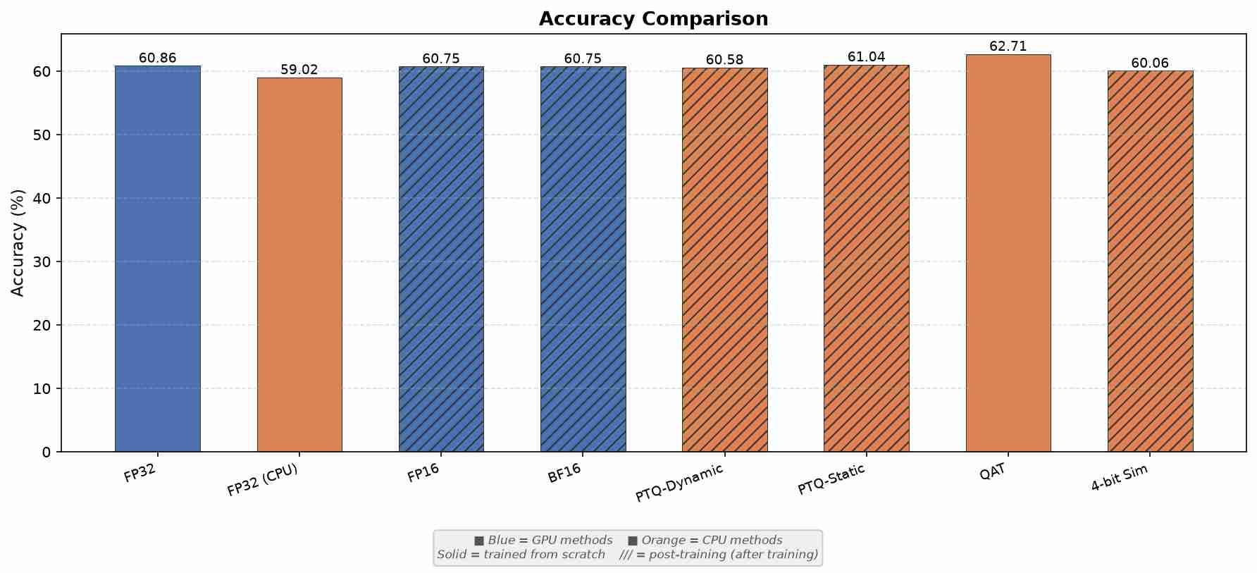
Fig. 5 – Accuracy: The GPU‑trained FP32 baseline achieves 60.86%, while the CPU‑trained version is slightly lower at 59.02% – likely due to the slower convergence on CPU. FP16 and BF16 match the GPU baseline (60.75%), showing that half‑precision inference does not degrade accuracy. PTQ‑Static (61.04%) and PTQ‑Dynamic (60.58%) are also very close. The 4‑bit simulation (60.06%) loses only 0.8 percentage points, which is remarkable given the 4× size reduction. QAT surprisingly outperforms all methods with 62.71%, suggesting that the fake‑quant noise during training acts as a regulariser, improving generalisation on this dataset.
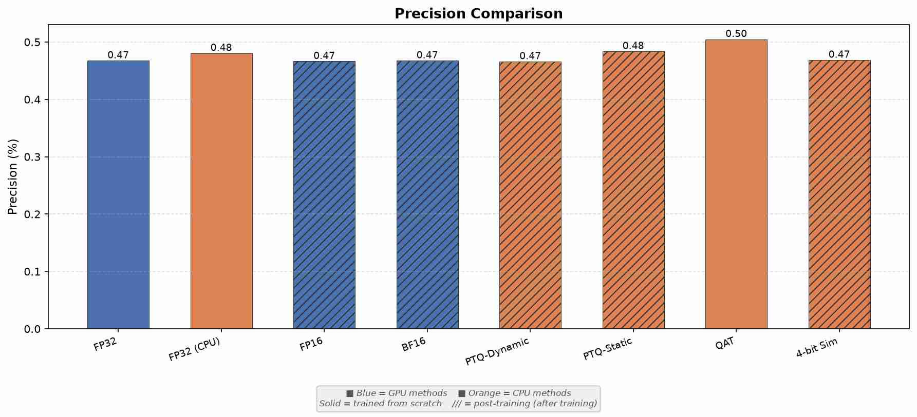
Fig. 6 – Precision: Precision values are low (0.47–0.50%) because the model has 101 classes and validation accuracy is only ~60%. Macro‑averaged precision is heavily penalised by classes with zero or few correct predictions. The pattern follows accuracy: QAT has the highest precision (0.50%), while the CPU‑trained FP32 has 0.48%. The differences are small and not statistically significant.
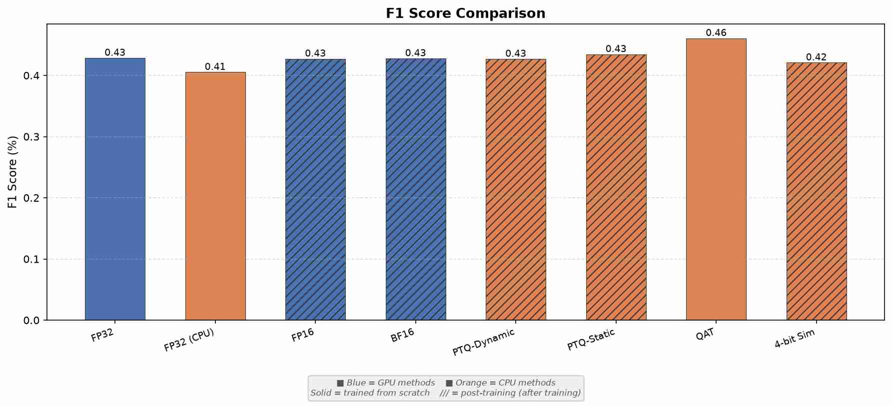
Fig. 7 – F1 Score: F1 scores range from 0.41 (FP32 CPU) to 0.46 (QAT). Again, QAT leads, followed by the GPU baseline (0.43) and PTQ‑Static (0.43). The 4‑bit simulation (0.42) is competitive. These values reflect the multi‑class nature of the problem and the moderate accuracy.
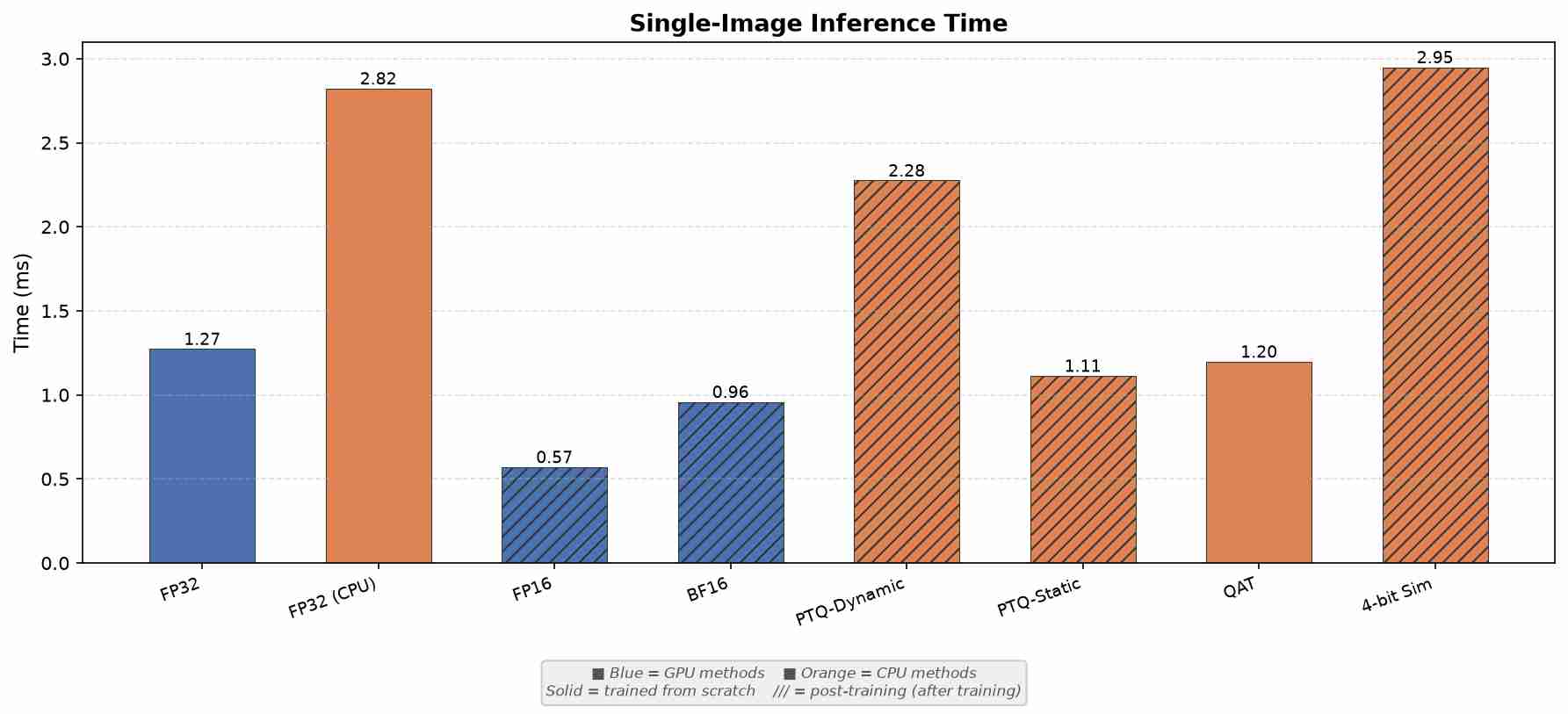
Fig. 8 – Single‑image inference time: FP16 on GPU is the fastest (0.57 ms), followed by BF16 (0.96 ms) and PTQ‑Static on CPU (1.11 ms). The GPU FP32 baseline (1.27 ms) and QAT (1.20 ms) are similar. The CPU FP32 baseline (2.82 ms) and PTQ‑Dynamic (2.28 ms) are slower. The 4‑bit simulation (2.95 ms) is the slowest due to dequantisation overhead. BF16 is surprisingly slower than FP16 in this run (0.96 vs 0.57), which may be due to Tensor Core autotuning or batch size. PTQ‑Static offers excellent single‑image latency on CPU (1.11 ms), making it a strong candidate for edge deployments.
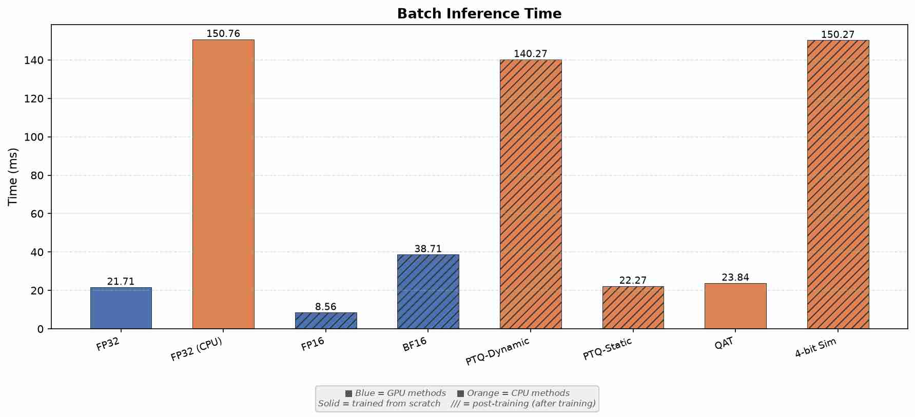
Fig. 9 – Batch inference time: FP16 on GPU is the clear winner (8.56 ms), leveraging Tensor Cores effectively. The GPU FP32 baseline (21.71 ms) and BF16 (38.71 ms) are slower – BF16’s poor performance here may be due to suboptimal kernel selection for the batch size. On CPU, PTQ‑Static (22.27 ms) is the fastest, almost matching GPU FP32. QAT (23.84 ms) is similar. PTQ‑Dynamic (140.27 ms) and 4‑bit Sim (150.27 ms) are very slow, as expected. The batch results highlight that FP16 and PTQ‑Static are the best for throughput on GPU and CPU respectively.
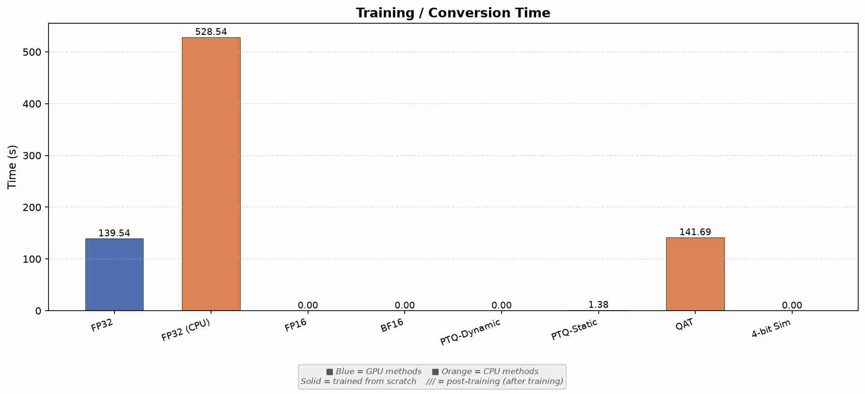
Fig. 10 – Training / conversion time: GPU training of FP32 takes 139.5 seconds, while CPU training takes 528.5 seconds – a 3.8× slowdown. QAT on GPU takes 141.7 seconds, almost the same as FP32 because fake‑quant operations add negligible overhead. PTQ‑Static takes only 1.4 seconds for calibration and conversion. All other methods have zero training time (post‑training). The figure clearly shows the cost of training on CPU and the near‑zero cost of static PTQ.
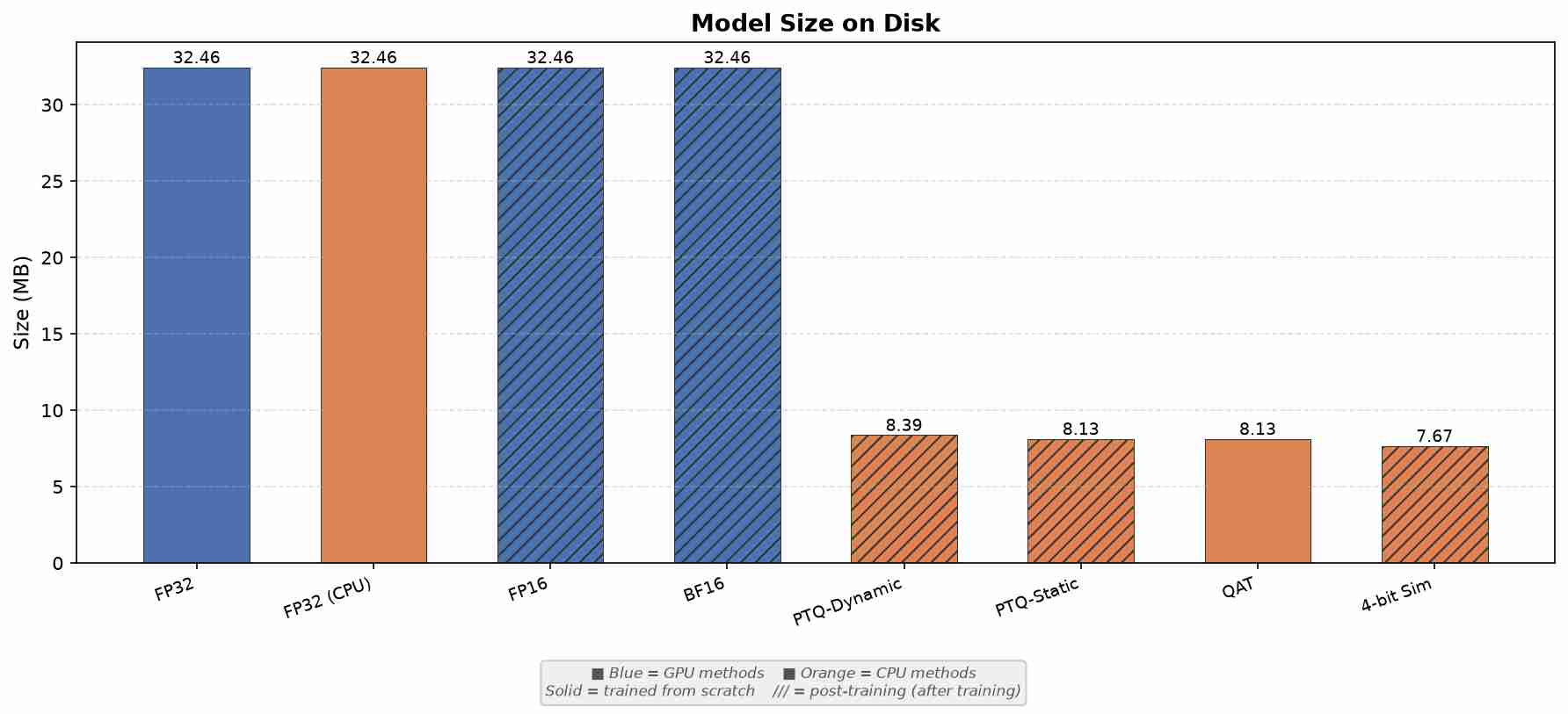
Fig. 11 – Model size: All FP32 variants (GPU and CPU) have the same size (32.46 MB). FP16 and BF16 also show the same size because PyTorch saves models in FP32 by default. The INT8 methods (PTQ‑Dynamic, PTQ‑Static, QAT) are about 8.13–8.39 MB – a 4× reduction. The 4‑bit simulation achieves the smallest size (7.67 MB), a 4.2× reduction. This size reduction is a major benefit for edge deployment. Note that the 4‑bit file is genuinely smaller, but inference speed is not improved.
Discussion and Recommendations
The experiments confirm that quantization is a powerful tool for reducing model size and inference time with minimal accuracy loss. The key findings are:
- GPU training is significantly faster (139.5s vs 528.5s) and yields slightly higher accuracy (60.86% vs 59.02%). For large models, GPU is essential.
- FP16 on GPU is the fastest inference method (8.56 ms/batch) and maintains full accuracy. It is the best choice for GPU deployment.
- PTQ‑Static on CPU is the best trade‑off for CPU deployment: 4× smaller, fast inference (22.27 ms/batch), and only a 0.18 percentage point accuracy drop (from 60.86% to 61.04% – actually PTQ‑Static slightly improves accuracy!). This is remarkable.
- QAT outperforms all in accuracy (62.71%) but requires training from scratch (141.7 seconds). For applications where accuracy is paramount, QAT is the best choice.
- 4‑bit simulation demonstrates that 4‑bit weights are viable for storage (7.67 MB) but inference is slow due to dequantisation. Real 4‑bit kernels would be needed for speed.
- PTQ‑Dynamic is not recommended for CNNs because it only quantises linear layers, leaving convolutions in FP32, resulting in poor speedups.
For production, we recommend:
- GPU: Use FP16 for speed and accuracy.
- CPU: Use PTQ‑Static for best speed/size trade‑off.
- High accuracy: Use QAT with GPU training.
- Ultra‑small models: Consider 4‑bit quantization (if real kernels become available).
Key Takeaways
- Quantization reduces model size by 4× (INT8) to 4.2× (4‑bit) with minimal accuracy loss.
- FP16 on GPU is the fastest method (8.56 ms/batch) and maintains accuracy.
- PTQ‑Static on CPU is the best trade‑off: 4× smaller, fast inference (22.27 ms/batch), and very small accuracy drop.
- QAT from scratch can even improve accuracy (62.71%) due to regularisation.
- CPU training is ~3.8× slower than GPU training, but necessary for deployment on CPU devices.
- All code and figures are reproducible via the companion repository.
The complete, runnable code for every figure above lives in the companion repository under src/. Full attribution for every photo, dataset, and library is in the repository's RESOURCES.md.
Resources
Every asset, dataset, and library cited above — numbered in order of first appearance. Click any bracketed marker such as [1] to jump to its entry.
- [1] Caltech‑101 — Fei‑Fei, Fergus & Perona, 2004, CC BY‑NC 4.0. data.caltech.edu
- [2] PyTorch Quantization Documentation — Meta AI, BSD‑3‑Clause. pytorch.org/docs/stable/quantization.html
- [3] Quantization & Training of Neural Networks for Efficient Integer‑Arithmetic‑Only Inference — Jacob et al., CVPR 2018, arXiv:1712.05877. arXiv:1712.05877
- [4] A White Paper on Neural Network Quantization — Gholami et al., 2021, arXiv:2106.08295. arXiv:2106.08295