A ResNet-50 looks at a photo of a white husky[18] sitting in the grass beside a child and can't make up its mind: Eskimo dog, 11%; Siberian husky, 6%; the rest of its confidence scattered across dozens of other breeds. Is the network actually looking at the dog, or at the child next to it? A plain accuracy number will never tell you. A Class Activation Map (CAM) will: it paints a heatmap over the exact pixels that pushed the model toward a class. This article uses Torch-CAM[1] to generate those heatmaps for four different networks and then puts them to work debugging a confused classifier.
{readmore}What is a Class Activation Map?
A convolutional network keeps spatial information almost all the way to the end. The last convolutional block outputs a stack of feature maps — small grids (say 7×7) where each channel has learned to respond to some pattern. A CAM answers one question: for the class the model chose, which locations in that grid mattered, and how much?
Different CAM variants estimate that "how much" differently. The original CAM[2] reads the weights of a global-average-pool + linear head directly. Gradient methods like Grad-CAM[3], Grad-CAM++[4], SmoothGradCAM++[5] and Layer-CAM[6] instead backpropagate the class score into the feature maps and use the gradients as importance weights — which means they work on almost any CNN. Torch-CAM implements all of them behind one small, consistent API.
Setup
python -m venv .venv
.venv\Scripts\activate            # Windows
pip install -r requirements.txt   # torch, torchvision, torchcam, matplotlib, pillow

# For an NVIDIA GPU, install the CUDA build of PyTorch instead:
pip install torch torchvision --index-url https://download.pytorch.org/whl/cu126
Line 1 creates the virtual environment; line 2 activates it on Windows; line 3 installs the CPU dependencies; lines 5–6 are the alternative one-line install of the CUDA build for an NVIDIA GPU.
The stack is PyTorch[7] and torchvision[8] for the models and weights, Torch-CAM[1] for the maps, and Matplotlib[9] plus Pillow[10] for rendering and image I/O. Every script runs from the project root so the relative assets/ paths resolve, and each one automatically uses CUDA when it is available and falls back to CPU otherwise:
import torch

def pick_device():
    return torch.device("cuda" if torch.cuda.is_available() else "cpu")
Line 1 imports torch; lines 3–4 define pick_device(), which returns a CUDA device when one is available and falls back to the CPU otherwise.
The Torch-CAM pipeline
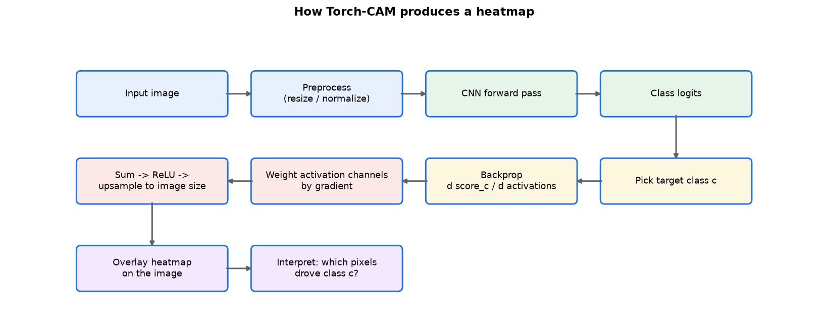
The pipeline in Fig 1 is the backbone of every example that follows. Three helpers, shared by all of them, cover the boring parts: preprocessing an image the way an ImageNet[11] model expects, and painting the returned activation map back onto the picture. Torch-CAM's overlay_mask does the actual blending.
from torchvision import transforms
from torchvision.transforms.functional import to_pil_image
from torchcam.utils import overlay_mask

IMAGENET_MEAN = (0.485, 0.456, 0.406)
IMAGENET_STD = (0.229, 0.224, 0.225)

def preprocess(pil_img, size=224):
    transform = transforms.Compose([
        transforms.Resize(size),
        transforms.CenterCrop(size),
        transforms.ToTensor(),
        transforms.Normalize(mean=IMAGENET_MEAN, std=IMAGENET_STD),
    ])
    return transform(pil_img).unsqueeze(0)          # add the batch dimension

def make_overlay(display_img, activation_map, alpha=0.5):
    mask = to_pil_image(activation_map.detach().cpu(), mode="F")
    return overlay_mask(display_img, mask, alpha=alpha)
Lines 1–3 import the transforms, the tensor→PIL helper, and Torch-CAM's overlay_mask; lines 5–6 hold the ImageNet normalization constants; lines 8–15 define preprocess(), which resizes, center-crops, tensorizes and normalizes the image, then adds a batch dimension (line 15); lines 17–19 define make_overlay(), converting the activation map to a single-channel image (line 18) and blending it over the picture (line 19).
Example 1 — ResNet-18 with SmoothGradCAM++
The simplest case. You never have to name a target layer: Torch-CAM inspects the model and hooks the last convolutional stage automatically. SmoothGradCAM++ averages the map over several noisy copies of the input, which tends to give a cleaner heatmap than plain Grad-CAM.
from torchvision.models import resnet18, ResNet18_Weights
from torchcam.methods import SmoothGradCAMpp

weights = ResNet18_Weights.IMAGENET1K_V1
labels = weights.meta["categories"]
model = resnet18(weights=weights).to(device).eval()

input_tensor = preprocess(pil_img=load_image(path="assets/inputs/dog.jpg")).to(device)

cam_extractor = SmoothGradCAMpp(model)          # target layer auto-detected
scores = model(input_tensor)
class_idx = int(scores.squeeze(0).argmax().item())
activation_map = cam_extractor(class_idx, scores)[0].squeeze(0)
cam_extractor.remove_hooks()                    # always detach the forward/backward hooks
Lines 1–2 import the model and the CAM method; lines 4–6 load the pretrained weights, read the category labels, and build the model in eval mode; line 8 preprocesses the dog photo; line 10 constructs the extractor (auto-detecting the target layer); line 11 runs the forward pass; line 12 picks the top-1 class; line 13 computes that class's activation map; line 14 removes the hooks.
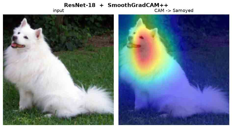
The overlay in Fig 2 shows the payoff: the heat sits on the animal. Two details matter and repeat in every example. First, the extractor needs the raw scores tensor from the forward pass, not a detached copy, because it backpropagates through it. Second, always call remove_hooks() when you are done — the extractor installs forward and backward hooks on the model, and leaving them attached will corrupt later inference.
Example 2 — MobileNet-V2 with Grad-CAM (naming the layer)
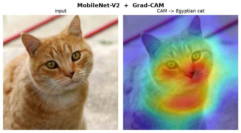
Auto-detection does not fit every architecture, so Torch-CAM lets you point the extractor at an explicit module. Here we hand plain Grad-CAM the whole model.features block as its target layer; the resulting map is shown in Fig 3.
from torchvision.models import mobilenet_v2, MobileNet_V2_Weights
from torchcam.methods import GradCAM

weights = MobileNet_V2_Weights.IMAGENET1K_V1
model = mobilenet_v2(weights=weights).to(device).eval()

cam_extractor = GradCAM(model, target_layer=model.features)
scores = model(input_tensor)
class_idx = int(scores.squeeze(0).argmax().item())
activation_map = cam_extractor(class_idx, scores)[0].squeeze(0)
cam_extractor.remove_hooks()
Lines 1–2 import MobileNet-V2 and Grad-CAM; lines 4–5 load the weights and build the model; line 7 points the extractor at model.features explicitly; lines 8–10 run the forward pass, take the top-1 class, and extract its map; line 11 removes the hooks.
Example 3 — VGG-16 with Layer-CAM
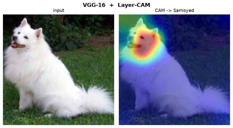
VGG-16 is a deep, plain convolutional stack, and Grad-CAM's single global weight per channel can look blurry on it. Layer-CAM weights each spatial location by its positive gradient, producing a noticeably sharper map on this kind of network — you can see the extra sharpness in Fig 4.
from torchvision.models import vgg16, VGG16_Weights
from torchcam.methods import LayerCAM

weights = VGG16_Weights.IMAGENET1K_V1
model = vgg16(weights=weights).to(device).eval()

cam_extractor = LayerCAM(model, target_layer=model.features)
scores = model(input_tensor)
class_idx = int(scores.squeeze(0).argmax().item())
activation_map = cam_extractor(class_idx, scores)[0].squeeze(0)
cam_extractor.remove_hooks()
Lines 1–2 import VGG-16 and Layer-CAM; lines 4–5 load the weights and build the model; line 7 points the extractor at model.features; lines 8–10 run the forward pass, take the top-1 class, and extract its map; line 11 removes the hooks.
Example 4 — Your own CNN and the original CAM
The original CAM is almost free, but only if your model ends in a global average pool followed by a single linear layer. So we build a small CIFAR-10[17] network with exactly that head:
class Simple_CNN(nn.Module):
    def __init__(self, num_classes=10):
        super().__init__()
        self.features = nn.Sequential(
            nn.Conv2d(3, 32, 3, padding=1), nn.BatchNorm2d(32), nn.ReLU(inplace=True),
            nn.MaxPool2d(2),
            nn.Conv2d(32, 64, 3, padding=1), nn.BatchNorm2d(64), nn.ReLU(inplace=True),
            nn.MaxPool2d(2),
            nn.Conv2d(64, 128, 3, padding=1), nn.BatchNorm2d(128), nn.ReLU(inplace=True),
        )
        self.pool = nn.AdaptiveAvgPool2d(1)     # global average pool
        self.classifier = nn.Linear(128, num_classes)

    def forward(self, x):
        x = self.features(x)
        x = self.pool(x)
        x = torch.flatten(x, 1)
        return self.classifier(x)
Lines 4–10 stack three convolution→batch-norm→ReLU blocks with max-pooling between them; line 11 is the global average pool and line 12 the single linear head — exactly the GAP+FC shape the original CAM needs; lines 14–18 define the forward pass: features (line 15), pool (line 16), flatten (line 17), classify (line 18).
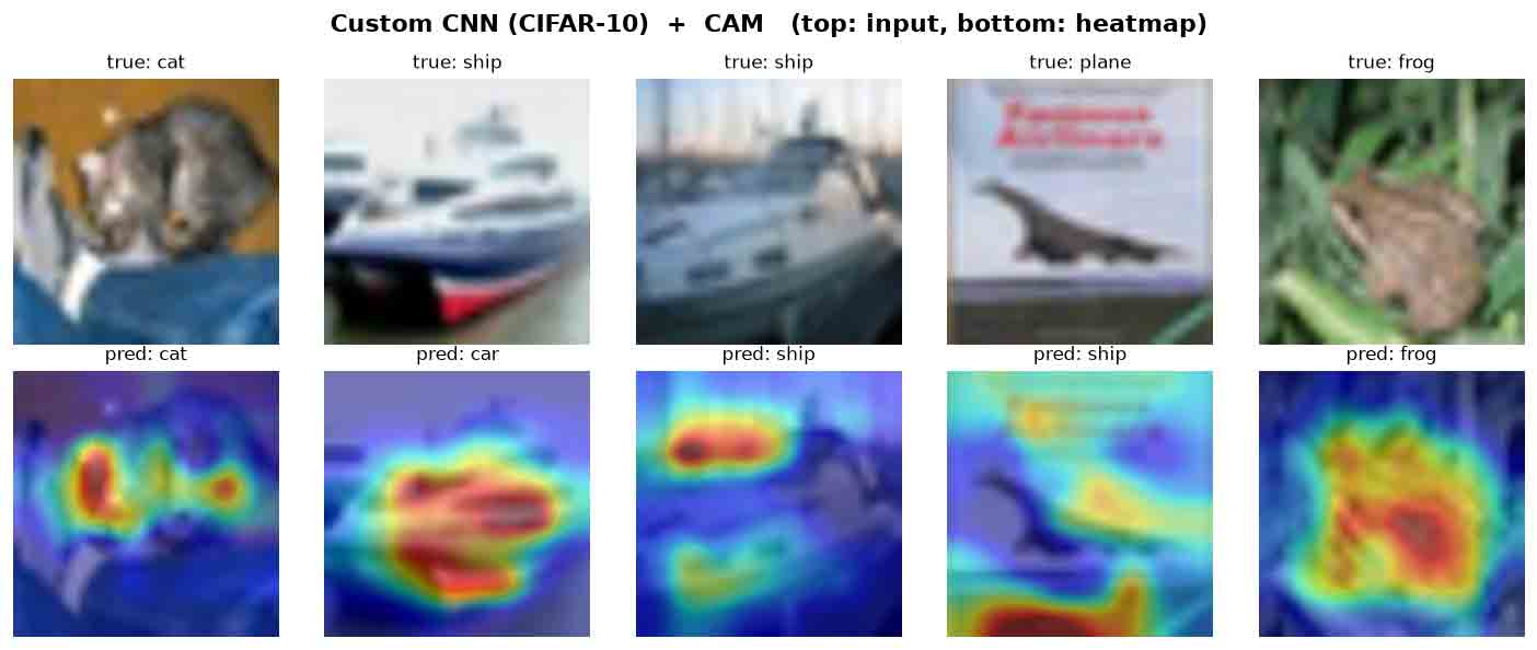
Train it for a few epochs (python src/train_custom_cnn.py saves the weights to checkpoints/simple_cnn.pt), then attach the CAM extractor by naming the feature block and the fully-connected head. Because the weights are the importance weights, no backward pass is needed. The maps for five test images appear in Fig 5.
from torchcam.methods import CAM

model = Simple_CNN().to(device)
model.load_state_dict(torch.load("checkpoints/simple_cnn.pt", map_location=device))
model.eval()

cam_extractor = CAM(model, target_layer="features", fc_layer="classifier")
scores = model(input_tensor)
class_idx = int(scores.squeeze(0).argmax().item())
activation_map = cam_extractor(class_idx, scores)[0].squeeze(0)
Line 1 imports CAM; lines 3–5 instantiate the model, load the trained weights, and switch to eval mode; line 7 attaches the extractor by naming the feature block and the FC head (no backward pass needed); lines 8–10 run the forward pass, take the top-1 class, and read off its map.
Putting CAMs to work: debugging a confused classifier
This is where CAMs earn their keep. A strong model often splits its confidence between two visually similar classes. Instead of computing one heatmap, compute a separate CAM for each of the top-2 classes and compare where the model looks for each label.
from torchvision.models import resnet50, ResNet50_Weights
from torchcam.methods import GradCAM

model = resnet50(weights=ResNet50_Weights.IMAGENET1K_V2).to(device).eval()

probabilities = model(input_tensor).softmax(1).squeeze(0)
top_prob, top_idx = probabilities.topk(3)       # inspect the competing classes

cam_extractor = GradCAM(model, target_layer=model.layer4)
for rank in range(2):                           # a CAM for each of the top-2 classes
    class_idx = int(top_idx[rank].item())
    scores = model(input_tensor)
    activation_map = cam_extractor(class_idx, scores)[0].squeeze(0)
    # overlay activation_map for this class ...
cam_extractor.remove_hooks()
Lines 1–2 import ResNet-50 and Grad-CAM; line 4 builds the model; lines 6–7 compute the softmax probabilities and pull the top-3 competing classes; line 9 constructs a single extractor on model.layer4; lines 10–14 loop over the top-2 classes, re-running the forward pass (line 12) and extracting a separate map for each (line 13); line 15 removes the hooks once, after the loop.
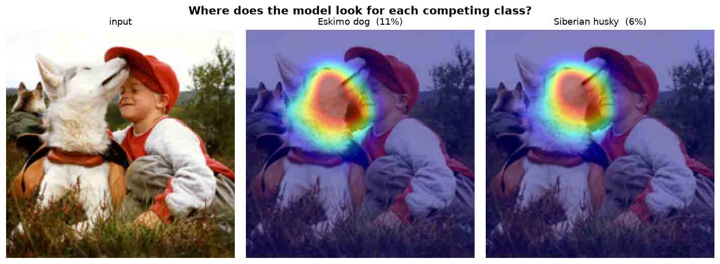
In Fig 6 both maps sit squarely on the dog's face — not the child, not the grass — so the hesitation is genuine class confusion between two near-identical breeds, not a background artifact. That is already a useful verdict: the fix is more discriminative training examples, not cleaner data. The two maps turn a vague "the model is confused" into a specific diagnosis, and the decision guide in Fig 7 summarizes how to read them in general:
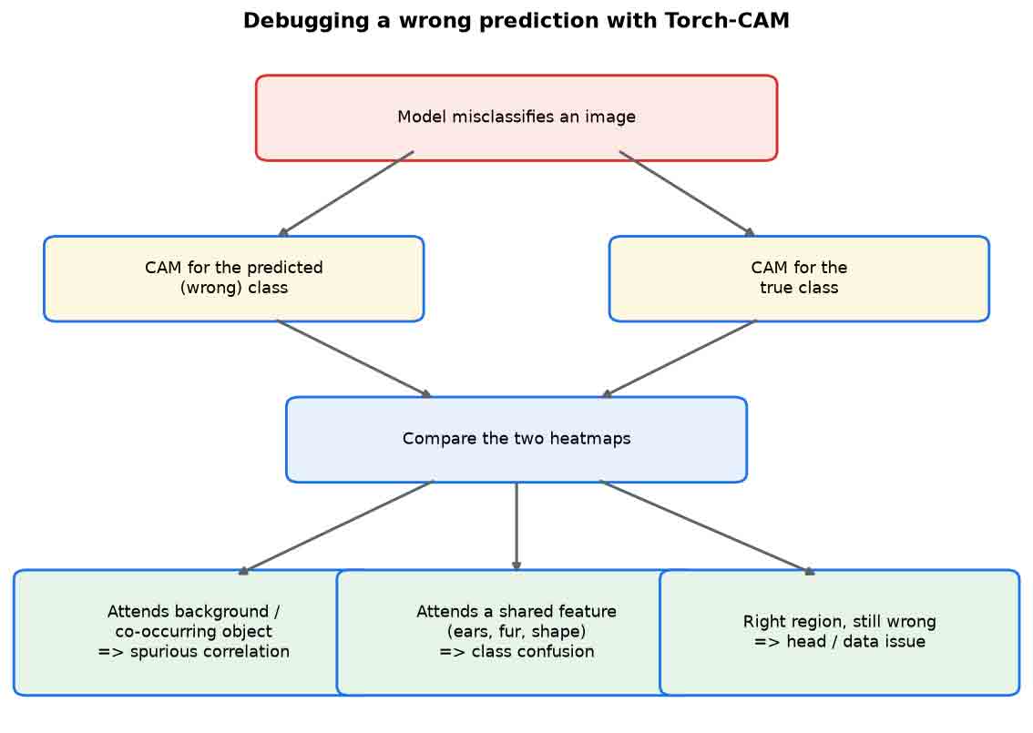
- It attends the background or a co-occurring object (snow, a hand, a leash) → the model latched onto a spurious correlation; fix the data.
- Both classes light up the same shared feature (ears, fur, silhouette) → genuine class confusion; you need more discriminative examples.
- It looks at the right region but still gets it wrong → the problem is downstream in the classifier head or the labels, not the features.
Probing a class's bias: the ibex and the saxophone
There is a second, sneakier way to use the same trick. Nothing forces you to pass the predicted class index to the extractor — you can hand it any class and ask: what in this image would count as evidence for that label? That turns a CAM from an explanation into a probe of what a class channel has actually learned.
A well-known example from the interpretability literature: ImageNet models identify an ibex chiefly by its enormous ridged, curled horns. Run the ibex-class CAM on a real ibex[19] and the heat sits on the head and horns — that one spiral feature carries the class. The flip side is that other spiral shapes can excite the same channel: a saxophone's curved bow and bell, a corkscrew, a French horn. Force the ibex CAM onto a saxophone[20] photo and watch where it lands:
ibex_idx = labels.index("ibex")                 # probe a class we did NOT predict

cam_extractor = GradCAM(model, target_layer=model.layer4)
scores = model(sax_tensor)                      # a saxophone, classified as "sax" (59%)
activation_map = cam_extractor(ibex_idx, scores)[0].squeeze(0)   # ...but ask about "ibex"
cam_extractor.remove_hooks()
Line 1 looks up the ibex class index — a class we did not predict; line 3 builds the extractor; line 4 runs the forward pass on the saxophone; line 5 forces the map for the ibex class instead of the prediction; line 6 removes the hooks.
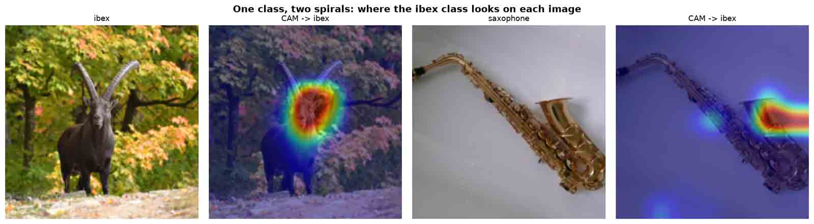
As Fig 8 shows, on this clean studio shot the model is not fooled — it says sax at 59% and ibex ranks a distant #721 — but the heatmap shows exactly where an ibex mistake would come from. In a harder photo (odd angle, clutter, an arm wrapped around the instrument hiding the keywork) that spiral evidence is what pulls the prediction toward the animal. This is the CAM-as-probe pattern: pick a class you are worried about, force its map, and you get a picture of the shape bias the network attached to that label — before it ever costs you a misclassification in production.
When the right class doesn't exist: a gallery of true misclassifications
The saxophone above was never actually misclassified — we forced the ibex map to expose the bias. So what does a CAM look like on a mistake the model really makes? The most reliable way to produce one is to show the network a subject that has no class at all in its label set. ImageNet-1k has no giraffe, no hedgehog, no dolphin, no raccoon, no tortoise. The model cannot answer "none of the above"; it is forced onto the nearest label it does know, and the CAM on that wrong class reveals which feature dragged it there.
scores = model(input_tensor)                     # a giraffe photo...
pred_idx = int(scores.softmax(1).argmax().item())    # ...top-1 comes back "cheetah"

cam_extractor = GradCAM(model, target_layer=model.layer4)
activation_map = cam_extractor(pred_idx, scores)[0].squeeze(0)   # CAM on the WRONG class
cam_extractor.remove_hooks()
Line 1 runs the forward pass on the giraffe photo; line 2 takes the (wrong) top-1 class, cheetah; line 4 builds the extractor; line 5 computes the CAM for that wrong class; line 6 removes the hooks.
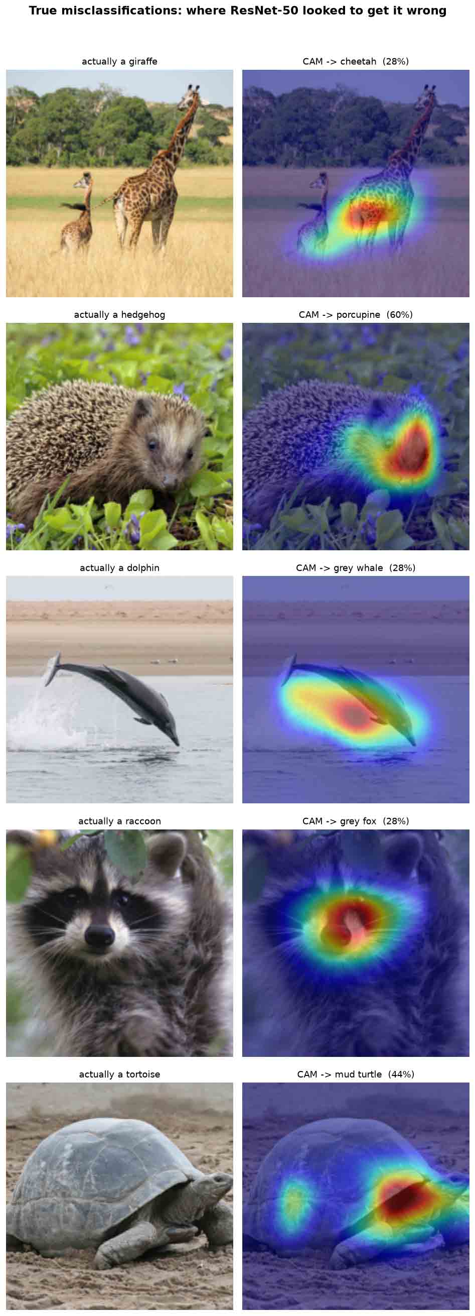
None of the five errors in Fig 9 is a random slip. In every case the network locked onto the single most salient feature it associates with a class it does know — and the heatmap points straight at it:
- Giraffe[21] → cheetah (28%). The map sits on the flank, not the long neck or the tall legs. A giraffe's brown-on-cream blotches read as the dark-spot-on-tan coat of the only spotted cats ImageNet knows — cheetah and leopard. This is textbook CNN texture bias[26]: the coat pattern outweighs the unmistakable giraffe silhouette.
- Hedgehog[22] → porcupine (60%) — the most confident error of the five. The heat blankets the spiny back. Porcupine is ImageNet's one spine-covered mammal, and at the level of local texture a field of quills is a field of quills.
- Dolphin[23] → grey whale (28%). The map wraps the smooth grey body. With no "dolphin" class available, a mid-leap fusiform body and dorsal fin over water fall onto the nearest cetacean — a whale. Body shape plus the water context do the damage.
- Raccoon[24] → grey fox (28%). Tellingly, the heat keys on the muzzle and grizzled fur and ignores the black eye-mask — the very feature a human would use to name it. A generic pointed-snout carnivore face is enough to drop it into the fox group.
- Tortoise[25] → mud turtle (44%). The map covers the domed carapace. Every testudine class in ImageNet is an aquatic turtle; a giant land tortoise collapses onto the closest one by shell shape.
Two distinct failure modes hide in that list, and the CAM tells them apart. Some errors are open-set — the true class simply does not exist, so some mistake is unavoidable and the only useful question is whether the model failed for a sensible reason. Others betray texture-over-shape bias — the giraffe and the hedgehog would be easy if the network weighted global shape as heavily as local texture, a well-documented CNN weakness. Either way, the heatmap turns a bare wrong label into a visual explanation you can act on: broaden the label set, add hard training examples, or reach for a more shape-biased backbone.
Which CAM method should I use?
| Method | Needs a backward pass? | Best for | In this project |
|---|---|---|---|
| CAM | No | Models with a global-avg-pool + linear head | Custom Simple_CNN |
| GradCAM | Yes | General-purpose default, any CNN | MobileNet-V2, ResNet-50 |
| SmoothGradCAMpp | Yes | Cleaner maps, multiple object instances | ResNet-18 |
| LayerCAM | Yes | Sharp, fine detail on deep plain stacks | VGG-16 |
Key takeaways
- Torch-CAM wraps every CAM variant in the same three-line pattern: construct the extractor → forward pass → call it with a class index and the scores.
- Let it auto-detect the layer when it can (ResNet); otherwise pass target_layer explicitly.
- Pick the method to match the architecture — CAM for a GAP+FC head, LayerCAM for sharp detail on deep plain stacks, GradCAM as the safe default.
- Always call remove_hooks() so the instrumented model behaves normally afterward.
- The real payoff is debugging: a per-class heatmap turns "wrong prediction" into an actionable cause — bad data, class confusion, or a head/label problem.
- The extractor accepts any class index, not just the prediction — force a class you are worried about to expose its learned shape bias (spiral ⇒ ibex).
- When the true category is missing from the label set the model must guess the nearest class it knows; the CAM shows whether it failed for a sensible reason — a shared coat, shell, or silhouette — and exposes the classic texture-over-shape bias.
The complete, runnable code for every figure above — four pretrained models, a trained-from-scratch CNN, the confused-classifier debugger, the ibex/saxophone class-bias probe, and the gallery of true misclassifications — lives in the companion repository under src/. Full attribution for every photo, dataset, and library is in the repository's RESOURCES.md.
Resources
Every photo, model, dataset, and library cited above — numbered in order of first appearance. Sample photos are used under the license noted for each; the CAM overlays in this article are derivative works of them. Click any bracketed marker such as [1] in the text to jump to its entry here.
- [1] Torch-CAM — F.-G. Fernandez, class activation explorer (Apache-2.0). github.com/frgfm/torch-cam
- [2] CAM — Zhou et al., Learning Deep Features for Discriminative Localization, CVPR 2016. arXiv:1512.04150
- [3] Grad-CAM — Selvaraju et al., Visual Explanations from Deep Networks via Gradient-based Localization, ICCV 2017. arXiv:1610.02391
- [4] Grad-CAM++ — Chattopadhay et al., WACV 2018. arXiv:1710.11063
- [5] Smooth Grad-CAM++ — Omeiza et al., 2019. arXiv:1908.01224
- [6] Layer-CAM — Jiang et al., Exploring Hierarchical Class Activation Maps for Localization, IEEE TIP 2021. IEEE Xplore
- [7] PyTorch — Paszke et al., An Imperative Style, High-Performance Deep Learning Library, NeurIPS 2019. pytorch.org
- [8] torchvision — pretrained models & transforms. github.com/pytorch/vision
- [9] Matplotlib — J. D. Hunter, Matplotlib: A 2D Graphics Environment, CiSE 2007. matplotlib.org
- [10] Pillow (PIL fork) — image I/O. python-pillow.org
- [11] ImageNet — Deng et al., CVPR 2009; Russakovsky et al., IJCV 2015. image-net.org
- [12] ResNet — He et al., Deep Residual Learning for Image Recognition, CVPR 2016. arXiv:1512.03385
- [13] Dog photo — PyTorch Hub sample (BSD-3-Clause). pytorch/hub
- [14] MobileNet-V2 — Sandler et al., Inverted Residuals and Linear Bottlenecks, CVPR 2018. arXiv:1801.04381
- [15] Cat photo — Fir0002 / Flagstaffotos, CC BY-NC 3.0 / GFDL 1.2. Wikimedia Commons
- [16] VGG — Simonyan & Zisserman, Very Deep Convolutional Networks for Large-Scale Image Recognition, ICLR 2015. arXiv:1409.1556
- [17] CIFAR-10 — Krizhevsky, Learning Multiple Layers of Features from Tiny Images, 2009. cs.toronto.edu/~kriz/cifar.html
- [18] Siberian husky photo — Per Harald Olsen (NTNU), CC BY-SA 3.0. Wikimedia Commons
- [19] Alpine ibex photo — DaPuglet, CC BY-SA 2.0. Wikimedia Commons
- [20] Alto saxophone photo — TR001, CC BY-SA 3.0. Wikimedia Commons
- [21] Giraffe photo — Lisa H via Unsplash, CC0 1.0 (public domain). Wikimedia Commons
- [22] European hedgehog photo — Michael Gäbler, CC BY-SA 3.0. Wikimedia Commons
- [23] Bottlenose dolphin photo — Giles Laurent, CC BY-SA 4.0. Wikimedia Commons
- [24] Raccoon photo — Bill Buchanan, U.S. Fish & Wildlife Service (public domain). Wikimedia Commons
- [25] Aldabra giant tortoise photo — Muhammad Mahdi Karim, GFDL 1.2. Wikimedia Commons
- [26] Texture bias — Geirhos et al., ImageNet-trained CNNs are biased towards texture…, ICLR 2019. arXiv:1811.12231