Reinforcement learning (RL) is the branch of machine learning concerned with how an intelligent agent ought to take actions in an environment so as to maximise some notion of cumulative reward. Unlike supervised learning, which infers a mapping from inputs to outputs using a fixed corpus of labelled examples, or unsupervised learning, which seeks hidden structure in unlabelled data, RL is fundamentally about sequential decision‑making under uncertainty. It is the computational counterpart of how humans and animals learn by trial and error: we try something, observe the outcome, and adjust our future behaviour accordingly. From the superhuman performance of AlphaGo in the game of Go to the real‑time control of autonomous vehicles, from personalised medical treatment regimens to the alignment of large language models via reinforcement learning from human feedback (RLHF), RL has emerged as the dominant framework for problems that require a sequence of interdependent decisions, where the consequences of an action may not be felt until much later. This article offers a comprehensive, self‑contained introduction to reinforcement learning: its formal foundations, the challenges that distinguish it from other learning paradigms, its canonical architectural components, a detailed algorithmic taxonomy, and its wide array of practical applications. We then turn to a complete worked example—the classic Frozen Lake environment from the Gymnasium suite—and solve it using tabular Q‑learning. Through this example, we dissect exactly why Frozen Lake is fundamentally intractable for classification or regression, why the temporal credit‑assignment problem is the core obstacle, and how RL's interactive, value‑based approach naturally surmounts it, especially when the environment becomes stochastic (slippery ice).
Code: https://github.com/babak-abad/introduction-to-reinforcement-learning
What Is Reinforcement Learning? A Formal Perspective
At its core, reinforcement learning is the study of goal‑directed learning from interaction. The agent is not told which actions to take, as in supervised learning; instead, it must discover which actions yield the most reward by trying them out. The agent's behaviour—its policy—evolves over time as it accumulates experience. The environment, which may be stochastic or deterministic, responds to the agent's actions by transitioning to a new state and emitting a scalar reward signal. The agent's sole objective is to maximise the total amount of reward it receives over the long run, not just the immediate payoff.
The standard mathematical framework for formalising RL problems is the Markov decision process (MDP). An MDP is a discrete‑time stochastic control process defined by the tuple (S, A, P, R, γ), where:
- S is a finite set of states that completely describe the environment at any given time step.
- A is a finite set of actions available to the agent.
- P is the state‑transition probability function, defined as P(s′ | s, a) = Pr{St+1 = s′ | St = s, At = a}, which captures the dynamics of the environment.
- R is the reward function, typically R(s, a) = 𝔼[Rt+1 | St = s, At = a], giving the expected immediate reward for taking action a in state s.
- γ ∈ [0, 1] is the discount factor that determines the present value of future rewards. A γ close to 0 makes the agent myopic (concerned only with immediate rewards), while γ close to 1 makes it far‑sighted, valuing long‑term returns.
The agent's goal is to find a policy π – a mapping from states to actions (or to a probability distribution over actions) – that maximises the expected discounted return:
Gt = Rt+1 + γ Rt+2 + γ2 Rt+3 + … = ∑k=0∞ γk Rt+k+1
This return encapsulates the core trade‑off that defines RL: immediate versus delayed gratification. An action that yields a small reward now might set the stage for much larger rewards later, and vice versa. The discount factor provides a convenient mathematical way to ensure that the infinite sum converges and that the agent's optimisation problem remains well‑posed.
Related Problems and the Fundamental Challenges of RL
Reinforcement learning is not a single algorithm but a broad class of problems characterised by several interrelated challenges that make them qualitatively different from supervised or unsupervised settings. Understanding these challenges is essential for appreciating why RL requires its own toolkit.
- Sequential decision‑making and non‑independence – In RL, actions are not independent trials. Each action alters the state of the environment, which in turn influences all future actions and rewards. This temporal structure means that the data the agent collects is highly correlated and non‑i.i.d. (independent and identically distributed), violating the assumptions that underpin most supervised learning theory.
- Delayed feedback and temporal credit assignment – Perhaps the most defining challenge of RL is that the reward signal for a particular action may arrive many steps later. The agent must solve the credit‑assignment problem: given a final outcome (success or failure), which of the many preceding actions deserve the credit or blame? This is akin to a student who receives a final exam grade weeks after completing the course – the grade alone does not tell which study habits were most effective.
- Exploration versus exploitation – The agent must constantly decide whether to continue with actions it already knows to be good (exploitation) or to try novel, untested actions that might lead to even better outcomes (exploration). This is a classic multi‑armed bandit dilemma, but exacerbated by the sequential nature of the problem: a bad exploratory action can set the agent back many steps, yet without exploration the agent may settle for a suboptimal policy. Striking the right balance is critical for sample efficiency and asymptotic performance.
- Partial observability and state estimation – In many real‑world scenarios, the agent does not have direct access to the full state of the environment. Instead, it receives observations that are incomplete or noisy. This turns the MDP into a partially observable Markov decision process (POMDP), where the agent must maintain a belief state or use memory to infer the hidden dynamics.
- Generalisation and function approximation – When the state or action space is large or continuous, the agent cannot tabulate values for every possible state‑action pair. It must generalise from seen states to unseen ones using function approximators such as neural networks, which introduces additional challenges in stability and convergence, as famously addressed by deep Q‑networks (DQN) with experience replay and target networks.
These challenges are not merely academic; they manifest in practical difficulties. For example, the exploration‑exploitation dilemma means that an RL agent might spend thousands of episodes flailing randomly before it stumbles upon a successful strategy. The credit‑assignment problem implies that naive reward shaping – artificially engineering rewards to guide the agent – can easily backfire and lead to unintended behaviours. Thus, RL algorithms must be designed with these fundamental trade‑offs in mind, and their performance is often measured not just by final performance but by sample complexity, stability, and robustness to hyperparameter settings.
The Role of Reinforcement Learning in the Machine Learning Landscape
Machine learning is traditionally partitioned into three broad paradigms, each answering a distinct question. Supervised learning addresses the question: “Given a set of input‑output pairs, can we learn a mapping that generalises to new inputs?” It is predictive and relies on immediate, per‑example feedback (the label). Unsupervised learning addresses: “What structure, patterns, or latent factors can we discover in unlabelled data?” It is descriptive and has no external feedback – the quality of the representation is evaluated by downstream tasks or by intrinsic metrics like reconstruction error or cluster coherence.
Reinforcement learning occupies a third, fundamentally different niche. It answers: “What action should I take now to maximise future cumulative reward?” This is prescriptive and interactive. The feedback is scalar, delayed, and dependent on the agent's own actions. In supervised learning, the data is static and the loss function is usually convex or at least well‑behaved; in RL, the data distribution shifts as the agent's policy changes (the non‑stationarity problem), and the objective (expected return) is non‑convex and often discontinuous. Moreover, RL does not require a dataset of optimal behaviour; it learns from scratch through interaction, which is both a strength (it can discover novel strategies) and a weakness (it can be extremely sample‑inefficient).
This distinction has profound practical implications. When we have a large dataset of expert demonstrations, we can use imitation learning (a supervised approach) to clone the expert's behaviour. However, imitation learning suffers from covariate shift – small errors compound over time because the agent never learns to recover from its own mistakes. RL, by contrast, learns a closed‑loop policy that is robust to its own errors, precisely because it experiences the consequences of its actions during training. This makes RL the method of choice for control problems where the agent must operate autonomously in a dynamic environment, even when expert data is available, as reinforcement learning from human feedback (RLHF) exemplifies in the context of language model alignment.
Applications of Reinforcement Learning: A Broad Survey
The versatility of RL is reflected in its ever‑growing list of successful applications across industries, many of which would be impossible to solve with conventional supervised or unsupervised techniques.
- Robotics and automation – RL enables robots to learn dexterous manipulation, dynamic locomotion (walking, running, jumping), and assembly operations entirely through trial and error. Unlike traditional control theory, which requires an accurate model of the robot's dynamics, model‑free RL can learn directly from raw sensor inputs (e.g., joint angles, torque readings, vision) and adapt to damage or changing environments.
- Game playing and strategy games – RL has achieved landmark successes in games with vast state spaces and long time horizons. AlphaGo and its successors (AlphaZero) defeated the world's best human players in Go, a game with more possible board configurations than atoms in the universe. Atari games, Chess, and Dota 2 have also fallen to RL agents that learned superhuman strategies purely from self‑play and sparse reward signals.
- Healthcare and personalised medicine – RL is being applied to optimise sequential treatment regimens for chronic diseases, where a clinician must decide on dosages, drug combinations, and timing based on a patient's evolving health indicators. By framing treatment as an MDP, RL can learn policies that maximise long‑term survival or quality‑of‑life metrics, adapting to each patient's unique response.
- Finance and algorithmic trading – Financial markets are a natural fit for RL because they involve sequential decisions under uncertainty, with delayed and noisy reward signals (profit and loss). RL agents can learn optimal portfolio rebalancing strategies, market‑making, and execution algorithms that adapt to changing market conditions without relying on strong parametric assumptions.
- Autonomous driving and transportation – Self‑driving cars must make a continuous stream of decisions – steering, acceleration, braking, lane changing – while interacting with other vehicles and pedestrians. RL, particularly in simulation, allows these systems to learn safe and efficient policies that handle edge cases that are too dangerous to explore on real roads.
- Natural language processing and AI alignment – Reinforcement learning from human feedback (RLHF) has become a cornerstone of modern large language model (LLM) training. Instead of training a model solely on next‑token prediction (supervised fine‑tuning), RLHF uses a reward model trained on human preferences to guide the LLM's behaviour, making it more helpful, harmless, and honest. This hybrid approach leverages RL to fine‑tune the model in a way that supervised loss cannot, as it aligns the model with qualitative, context‑dependent human values.
These applications share a common thread: they require decisions that are not isolated but part of a long chain, where the optimal choice at any moment depends on the future consequences of the present action. This is precisely the domain where RL excels and where static, non‑sequential methods fall short.
Reinforcement Learning Architecture: The Agent–Environment Interface
The architecture of any RL system is unified by the agent–environment interface. At every discrete time step t, the agent receives a representation of the environment's state St ∈ S. Based on this state, the agent selects an action At ∈ A. One time step later, the agent receives a numerical reward Rt+1 ∈ ℝ and a new state St+1. The agent then updates its internal knowledge – its policy, value function, or both – and the cycle repeats. This loop is the unifying abstraction for all RL algorithms, regardless of whether the environment is a simulated physics engine, a board game, or a real‑world robotic system.
Within this architecture, three distinct functional components are commonly identified: the policy, the value function, and, optionally, a model of the environment. The policy is the agent's behaviour rule; the value function estimates expected returns; and the model predicts the environment's dynamics. These components combine in diverse ways to define the major algorithmic families. The following section provides a comprehensive taxonomy of these families, detailing their theoretical distinctions, practical trade‑offs, and typical application domains.
Taxonomy of Reinforcement Learning Algorithms
The family of RL algorithms is remarkably diverse, and choosing the right algorithm for a given problem requires understanding the fundamental categorisations that define how an agent learns. The most important axes of classification are: whether the agent builds an explicit model of the environment (model‑based vs. model‑free); whether it learns a value function, a policy, or both (value‑based, policy‑based, or actor‑critic); whether it learns from its own current actions or from any past data (on‑policy vs. off‑policy); and whether it uses deep neural networks for function approximation (deep RL). Each approach has distinct theoretical properties, sample‑efficiency profiles, and suitability to different types of state and action spaces.
Model‑Based vs. Model‑Free Reinforcement Learning
The first major division separates algorithms according to whether they construct an explicit model of the environment's transition dynamics and reward function.
Model‑based RL attempts to learn the transition probability P(s′|s, a) and the reward function R(s, a) from experience, or assumes that the model is known a priori. With a learned or known model, the agent can plan: it can simulate hypothetical trajectories, perform lookahead searches, and use dynamic programming or Monte Carlo tree search (MCTS) to select actions without interacting with the real environment for every decision. The archetypal model‑based approach is Dyna, which interleaves real experience with simulated experience to accelerate learning. MCTS, the engine behind AlphaGo, is a prime example: it uses a forward model of the game to simulate thousands of future moves, evaluating their outcomes to select the best immediate action.
The primary advantage of model‑based RL is sample efficiency – because the agent can generate synthetic experience, it often requires far fewer interactions with the real environment to learn a good policy. This is invaluable in domains where real‑world interaction is expensive, dangerous, or slow, such as robotics, healthcare, or industrial control. However, the model itself must be learned, and any inaccuracies in the model can lead to model bias – the agent optimises its policy for the wrong dynamics, resulting in suboptimal or even dangerous behaviour in the real world. Model‑based methods also impose additional computational overhead for planning.
Model‑free RL, in contrast, does not attempt to learn a model of the environment. Instead, it learns directly from the stream of interactions, using trial‑and‑error to estimate value functions or policies without ever inferring the transition dynamics. Q‑learning, SARSA, REINFORCE, and Proximal Policy Optimisation (PPO) are all model‑free algorithms. They are simpler to implement, less prone to model bias, and often more robust in practice, especially when the environment is highly stochastic or difficult to model. The trade‑off is that they are notoriously sample‑hungry: the agent must collect vast amounts of experience, often millions of steps, to converge to a satisfactory policy. For domains like Atari games or simulated robotics where interaction is cheap (i.e., the environment is a fast simulator), model‑free methods are the dominant choice.
The choice between model‑based and model‑free is not binary; many algorithms sit on a spectrum. For instance, model‑predictive control (MPC) uses a short‑horizon planning loop with a known or learned model to select actions, replanning at every step. Conversely, off‑policy model‑free methods can be augmented with learned models for data augmentation (a technique known as model‑based policy optimisation, or MBPO). The decision hinges on the application: if a high‑fidelity simulator is available and compute is abundant, model‑based planning (e.g., in autonomous driving simulators) is often preferred; if the environment is black‑box, complex, and high‑dimensional (e.g., natural language interactions), model‑free methods like PPO or Q‑learning are more frequently deployed.
Value‑Based Methods
Value‑based methods focus on learning a value function – either the state‑value V(s) or, more commonly, the action‑value Q(s, a) – and then deriving the policy implicitly by choosing the action with the highest estimated value in each state. The canonical example is Q‑learning, which we use in our worked example. The policy is greedy with respect to the learned Q‑function: π(s) = argmaxa Q(s, a). In tabular settings with finite state and action spaces, Q‑learning converges to the optimal policy under mild conditions.
The strengths of value‑based methods are their relative simplicity, theoretical convergence guarantees (in the tabular case), and their sample efficiency when combined with experience replay. They are particularly well‑suited to problems with discrete action spaces of moderate size, such as board games, Atari games, and many grid‑world navigation tasks. The Deep Q‑Network (DQN), which combines Q‑learning with a deep neural network function approximator, achieved human‑level performance on a suite of Atari games using only raw pixel inputs, marking a watershed moment for deep RL.
However, value‑based methods have several limitations. First, they are not directly applicable to continuous action spaces because the argmax operation over a continuous domain is computationally intractable. Second, they can suffer from overestimation bias: because the max operator uses the same values to both select and evaluate an action, the Q‑estimates tend to be systematically over‑optimistic. This issue is mitigated by techniques like Double Q‑learning (used in Double DQN). Third, value‑based methods are often unstable when combined with non‑linear function approximation, requiring carefully designed interventions such as target networks and gradient clipping.
Typical applications of value‑based RL include recommendation systems (where the action is selecting the next item from a finite catalogue), traffic signal control, and any domain where the decision space is naturally discrete and the evaluation of an action's long‑term consequence is paramount.
Policy‑Based Methods
Policy‑based methods side‑step the value function entirely (or use it only for variance reduction) and directly optimise the policy parameters θ via gradient ascent on the expected return. The core of these methods is the policy gradient theorem, which provides an analytical expression for the gradient of the expected return with respect to the policy parameters. The simplest policy‑gradient algorithm is REINFORCE, which uses Monte Carlo estimates of the return to update the policy: θ ← θ + α ∇θ log πθ(a|s) Gt.
The most compelling advantage of policy‑based methods is their natural ability to handle continuous action spaces. Instead of searching over a high‑dimensional action space for the maximum Q‑value, the policy network directly outputs a probability distribution (e.g., the mean and variance of a Gaussian distribution) from which actions are sampled. This makes them the de facto choice for robotic control, continuous control tasks in physics simulators, and any domain where actions are real‑valued (e.g., torque, angles, control gains).
Policy‑based methods also support stochastic policies, which can be beneficial in adversarial or partially observable settings where randomness is a strategic advantage (e.g., in poker or cybersecurity games). Furthermore, they tend to have more stable convergence properties because policy updates are smooth and incremental, unlike the sometimes abrupt changes in greedy action selection in value‑based methods. However, they are often sample‑inefficient and suffer from high variance in gradient estimates, which can slow learning. Modern policy‑based algorithms, such as Proximal Policy Optimisation (PPO) and Trust Region Policy Optimisation (TRPO), introduce constraints on the policy update step to prevent destructive updates, making them remarkably stable and widely used in both academic research and industry. PPO, in particular, has become the workhorse for training LLMs via RLHF.
Applications of policy‑based RL abound in robotics (walking, grasping, drone navigation), continuous control (video game bots with analog controls), and any environment where the action space is high‑dimensional or where the optimal policy is inherently stochastic.
Actor‑Critic Methods
Actor‑critic methods elegantly combine the strengths of value‑based and policy‑based approaches. They maintain two separate entities: an actor, which is a policy network that proposes actions, and a critic, which is a value network that estimates the value function (typically the advantage function) to evaluate the actor's actions. At each step, the actor updates its policy parameters in the direction suggested by the critic, while the critic updates its value estimates using TD learning. The critic provides a low‑variance baseline that reduces the variance of the policy gradient, enabling more stable and data‑efficient learning than pure policy‑gradient methods.
The actor‑critic framework is incredibly flexible and has given rise to many state‑of‑the‑art algorithms. A2C (Advantage Actor‑Critic) and A3C (Asynchronous Advantage Actor‑Critic) use multiple parallel environments to decorrelate data and accelerate training. SAC (Soft Actor‑Critic) incorporates entropy maximisation to encourage exploration and has become a standard baseline for continuous control. DDPG (Deep Deterministic Policy Gradient) extends DQN to continuous actions by using a deterministic policy, while TD3 (Twin Delayed DDPG) improves upon DDPG by addressing overestimation bias.
Actor‑critic methods are widely regarded as the most powerful and generally applicable family of RL algorithms because they can handle both discrete and continuous action spaces, leverage the efficiency of value learning, and enjoy the stability of policy optimisation. Their primary drawback is the increased complexity: they require careful hyperparameter tuning and can be sensitive to the learning rates of the actor and critic, which must be balanced to maintain stable co‑adaptation. In practice, actor‑critic algorithms (especially PPO, which is often classified as an actor‑critic method despite its policy‑based roots) dominate modern RL benchmarks, including robotic locomotion, MuJoCo tasks, and complex strategy games.
On‑Policy vs. Off‑Policy Learning
An orthogonal but equally important classification concerns whether the learning algorithm updates its policy or value function using data generated by the current policy (on‑policy) or by any policy, potentially including past policies (off‑policy).
On‑policy methods, such as SARSA and PPO, learn the value function or policy that is consistent with the agent's current behaviour. They evaluate and improve the policy that is actually being used to explore the environment. This guarantees that the updates are always relevant to the current policy, which can lead to more stable learning and well‑behaved convergence properties. However, on‑policy methods cannot reuse old data because the policy that generated the data is no longer the current policy; this makes them highly sample‑inefficient. For instance, in PPO, even though it is an actor‑critic method, it restricts updates to the current policy using importance sampling ratios, making it effectively on‑policy.
Off‑policy methods, exemplified by Q‑learning and its deep extensions (DQN, SAC), learn the value of the optimal policy independently of the behaviour policy used to generate the data. Because they can learn from any experience – whether generated by random exploration, an expert, or a historical version of the agent – they can make use of experience replay: storing past transitions in a buffer and sampling them randomly to break temporal correlations and dramatically improve sample efficiency. This off‑policy property is one of the reasons DQN was able to learn from Atari pixels effectively. The downside is that off‑policy learning can be less stable and more prone to divergence when combined with function approximation, as the distribution of the data (the replay buffer) can differ significantly from the distribution induced by the current policy (the problem of distributional shift).
The choice between on‑policy and off‑policy often depends on the cost of data collection. In simulation where data is cheap, on‑policy algorithms like PPO are preferred for their stability. In real‑world applications where data is expensive and must be reused (e.g., robotics data collected over months), off‑policy algorithms like SAC are more attractive because they can reuse every single transition many times.
Deep Reinforcement Learning (DRL)
Deep reinforcement learning refers to the integration of deep neural networks as function approximators for policies, value functions, or environment models within an RL framework. When the state space is high‑dimensional, continuous, or perceptual (e.g., raw images, LiDAR point clouds, or audio spectrograms), tabular methods become infeasible. Deep neural networks can compress these high‑dimensional inputs into meaningful latent representations and approximate complex, non‑linear value functions or policies with remarkable fidelity.
However, deep RL introduces significant challenges beyond those of supervised deep learning. The data is non‑stationary because the policy changes over time, leading to shifts in the input distribution. The targets (TD targets) themselves depend on the Q‑network, creating a moving target problem that can cause divergence. Standard solutions include experience replay (to break correlations), target networks (to stabilise the target values), and gradient clipping (to prevent exploding gradients). In policy‑based deep RL, advantage normalisation and trust‑region constraints (as in PPO) are essential to keep updates within a safe range.
DRL has enabled the application of RL to previously intractable problems. DQN demonstrated that a single architecture could learn to play 49 different Atari games from raw pixels, achieving human‑level performance in many. AlphaGo combined deep neural networks for policy and value with MCTS, defeating the world champion in a game with a branching factor of over 200. In continuous control, DDPG and SAC enable quadruped robots to learn walk and run gaits directly from joint sensors. More recently, RLHF with deep language models has emerged as the dominant paradigm for aligning LLMs, using a deep reward model to optimise a deep policy network (the LLM) via PPO.
While DRL is incredibly powerful, it remains notoriously difficult to reproduce and debug. Hyperparameters that work for one environment often fail catastrophically on another. The sample complexity is often extreme – millions or even billions of environment steps – which limits its use in domains without fast simulators. Research into meta‑learning, transfer learning, and offline RL (learning purely from static datasets) aims to address these limitations, making DRL more practical for real‑world deployment.
Worked Example: Solving Frozen Lake with Tabular Q‑Learning
To ground these abstract concepts, we now walk through a complete, end‑to‑end RL solution to the Frozen Lake problem, a classic benchmark from the Gymnasium library (the maintained successor of OpenAI Gym). This example sits squarely in the model‑free, value‑based, off‑policy quadrant of our taxonomy: we use tabular Q‑learning, which does not build a model, learns an action‑value function, and updates from experiences generated by an exploratory behaviour policy (ε‑greedy) that is different from the greedy target policy. Before we present the solution, we must first characterise the environment and the nature of the data it produces, because this characterisation is precisely what makes the problem so challenging for supervised learning.
The Frozen Lake Environment and Its Data Characteristics
Frozen Lake is a grid‑world environment where the agent must navigate across a frozen lake from a start tile to a goal tile while avoiding holes. The lake is represented as a 4×4 or 8×8 grid; we will use the standard 4×4 version. The agent can move in four directions: up, down, left, and right. At each time step, the agent chooses an action, and the environment transitions to a new state according to the transition dynamics. The agent receives a reward of +1 when it reaches the goal, and 0 otherwise. If the agent falls into a hole, the episode terminates with a reward of 0 and the agent is reset to the start state. The episode also terminates after a fixed number of steps (default 100) to prevent infinite loops.
The environment has two variants: non‑slippery (deterministic) and slippery (stochastic). In the non‑slippery version, the agent's action is executed exactly as intended – moving left always moves one cell to the left, provided that cell is within the grid. In the slippery version, the ice is treacherous: with probability 1/3, the action succeeds; otherwise, the agent slips perpendicularly (for example, if trying to move up, it might slip left or right with equal probability). This stochasticity makes the problem substantially harder because the agent cannot perfectly control its movement, and it must learn a policy that is robust to uncertainty.
The grid layout for the 4×4 map (using the default `"FrozenLake-v1"` map) is:
S F F F
F H F H
F F F H
H F F G
where:
- S = start (top‑left corner, state 0).
- G = goal (bottom‑right corner, state 15).
- F = frozen (safe) tile.
- H = hole (fatal – falling ends the episode).
The state space is discrete: each cell is numbered from 0 to 15. The agent's observation is simply the integer index of its current cell. This is a finite MDP with 16 states and 4 actions. The action space is also discrete: 0=left, 1=down, 2=right, 3=up (the Gymnasium convention).
The reward function is sparse: the agent receives +1 only when it reaches the goal (state 15); all other transitions yield 0. This sparsity is even more extreme than in Mountain Car (where every step gave -1), because here the agent receives no negative feedback for wandering or falling into holes – it simply gets a terminal state with zero reward. The only positive signal comes at the very end of a successful episode. This makes credit assignment exceptionally difficult: the agent must figure out which sequence of actions, possibly dozens of steps long, led to the goal, despite having no intermediate feedback.
For supervised learning, this environment is essentially impossible. A classifier would need training data of (state, optimal action) pairs, but the optimal action at a given state is not uniquely defined: in the non‑slippery case, from state 0 (top‑left), the optimal first action is to move right or down (both are safe and lead toward the goal); in the slippery case, the optimal action depends on the stochastic transition probabilities, and there is no single deterministic action that guarantees success with 100% probability – the agent must learn a policy that maximises the probability of success, which is a probabilistic optimisation problem. Moreover, the “correct” action for a state in the slippery case is not a label that can be observed; it is defined by the Bellman optimality equation, which involves expectations over future outcomes. A supervised learner, even if given a dataset of successful trajectories, would see that the same state (e.g., state 5) may appear with different actions that all led to success eventually, because of the stochastic slips. The mapping from state to action is therefore not a function – it is a distribution over actions, which classification cannot represent.
Furthermore, the data stream in RL is non‑stationary and temporally correlated. As the policy improves, the distribution of visited states changes drastically. In early episodes, the agent falls into holes frequently and rarely reaches the goal; in later episodes, it navigates more skilfully. This covariate shift makes it difficult for any fixed supervised model to generalise. Finally, the absence of a labelled dataset means that the agent must generate its own experience through interaction – exactly what RL is designed for.
In summary, Frozen Lake is an excellent testbed because it has a small, discrete state space (so tabular Q‑learning is feasible), but it exhibits the core RL challenges: delayed rewards, stochastic transitions (when slippery), and the need for exploration. It is a perfect example of a task that is intractable for classification or regression but readily solvable with Q‑learning.
This non‑deterministic mapping from state to action is precisely what makes Frozen Lake a quintessential RL problem and a poor fit for supervised learning. To better understand the environment visually, the following figure provides a colour‑coded representation of the Frozen Lake grid, highlighting the start, holes, safe tiles, and goal.
Fig. 2 provides a direct visual representation of the Frozen Lake environment, which is the core of our worked example. The 4×4 grid contains exactly four distinct tile types: the start tile (S, coloured blue), frozen safe tiles (F, green), holes (H, red), and the goal tile (G, yellow). The agent begins at the top‑left corner (state 0) and must navigate to the bottom‑right corner (state 15) while avoiding the holes that are scattered throughout the grid. This layout is deliberately designed to create a non‑trivial path‑finding problem: the agent cannot simply move straight down and right because holes block several direct routes. Instead, it must learn to navigate around these obstacles, which forces the agent to explore multiple paths before discovering a successful one. In the non‑slippery (deterministic) version, the agent can eventually memorise a fixed sequence of actions that guarantees success every time. However, in the slippery (stochastic) version, the ice is treacherous – with probability 1/3, the agent's intended action is executed, but with probability 2/3 it slips perpendicularly (e.g., trying to move right may result in moving up or down instead). This stochasticity transforms the problem from a simple path‑finding exercise into a robust control task: the agent must learn a policy that maximises the probability of reaching the goal, not just a fixed route. The visual layout shown here is crucial for understanding why the problem is hard for classification or regression: the optimal action in a given cell is not a single label but depends on the agent's uncertainty about its own movement. A classifier, even if given a dataset of successful trajectories, would see that the same cell (e.g., the safe tile at state 6) may require different actions in different episodes because the stochastic slips change the optimal behaviour. This non‑deterministic mapping from state to action is precisely what makes Frozen Lake a quintessential RL problem and a poor fit for supervised learning.
Relating the SVG Diagram to the Real Frozen Lake GUI. The Gymnasium Frozen Lake environment is typically rendered in a text‑based or simple graphical user interface (GUI) that displays the grid with colour‑coded tiles. In the real GUI, the start tile appears as a letter "S" (often in blue or highlighted), the goal as a letter "G" (often in gold or green), the holes as dark or red cells marked with "H", and the frozen tiles as light or green cells marked with "F". The agent is usually represented as a small character (often a circle or a triangle) that moves across the grid. The SVG diagram in Fig. 2 is a stylised, clean representation of this exact GUI: it preserves the same 4×4 structure, the same labels (S, F, H, G), and the same colour coding (blue for start, green for safe, red for holes, gold for goal). The agent is not shown in the static diagram because the purpose is to display the environment layout, but when the environment is rendered during animation, the agent appears as a moving character on top of the grid. The SVG was created by translating the text‑based representation (the `S F F F / F H F H / F F F H / H F F G` ASCII grid) into a visual format, using distinct colours to make the tiles immediately distinguishable. The diagram also includes grid lines and rounded corners to mimic the polished look of the Gymnasium GUI, making it easy for readers to map between the textual description, the visual diagram, and the actual rendered environment they would see when running the code.
Q‑Learning: The Algorithm and Its Mathematical Foundations
We solve Frozen Lake using Q‑learning, one of the most widely used and understood model‑free, off‑policy RL algorithms. Q‑learning learns the optimal action‑value function Q* (s, a), which satisfies the Bellman optimality equation:
Q*(s, a) = ∑s' P(s'|s,a) [ R(s,a) + γ maxa' Q*(s', a') ]
Intuitively, this equation states that the value of taking action a in state s is the immediate reward plus the discounted value of the best action in the next state, averaged over possible next states according to the transition dynamics. Q‑learning bypasses the need to know P and R by using sample‑based updates. The agent interacts with the environment, collects transitions (s, a, r, s'), and updates its estimate of Q using:
Q(s, a) ← Q(s, a) + α [ r + γ maxa' Q(s', a') – Q(s, a) ]
where α ∈ (0, 1] is the learning rate that controls how much new information overrides old estimates. The term r + γ maxa' Q(s', a') is called the temporal‑difference (TD) target, and the difference between the target and the current estimate is the TD error. This update rule is off‑policy because it learns the value of the optimal policy independently of the agent's current policy; the max operator uses the greedy action in the next state, even if the agent did not take that action. This off‑policy property makes Q‑learning remarkably flexible and allows it to learn from data generated by any policy, including random exploration, as long as all state‑action pairs are visited infinitely often.
The pseudocode for Q‑learning is deceptively simple:
Initialize Q(s, a) arbitrarily for all s ∈ S, a ∈ A
For each episode:
    Initialize state s
    For each step of episode:
        Choose action a from s using policy derived from Q (e.g., ε‑greedy)
        Take action a, observe reward r and next state s'
        Q(s, a) ← Q(s, a) + α [ r + γ maxa' Q(s', a') – Q(s, a) ]
        s ← s'
    Until s is terminal
The ε‑greedy policy ensures exploration: with probability ε, the agent takes a random action; with probability 1‑ε, it takes the greedy action (the one with the highest Q‑value). This allows the agent to continue discovering better paths even as it exploits known good ones.
Implementation: Complete Project Code Walkthrough
The complete implementation is available in the companion repository. The project is organised into several Python modules, each serving a specific purpose. Below we present each file in logical sections with detailed explanations.
Configuration Module (config.py) – Part 1: Environment and Space Settings
# Environment settings
ENV_NAME = 'FrozenLake-v1'
IS_SLIPPERY = True

# State/action space (4x4 grid = 16 states, 4 actions)
N_STATES = 16
N_ACTIONS = 4
Explanation: This section defines the core environment parameters. ENV_NAME specifies the Gymnasium environment to use. IS_SLIPPERY controls whether the ice is stochastic (slippery) or deterministic. N_STATES is set to 16 (4×4 grid), and N_ACTIONS is set to 4 (up, down, left, right). These constants are imported by other modules to ensure consistency.
Configuration Module (config.py) – Part 2: Hyperparameters, Persistence, and Output Paths
# Hyperparameters
ALPHA = 0.1          # Learning rate
GAMMA = 0.99         # Discount factor
EPSILON = 0.5        # Initial exploration rate (high to discover the goal)
EPSILON_MIN = 0.01   # Minimum exploration rate
EPSILON_DECAY = 0.9995  # Multiplicative decay per episode
EPISODES = 20000
TEST_EPISODES = 100

# Output directory for all generated artifacts
OUTPUT_DIR = 'outputs'

# Persistence – per-environment Q-table pickles
Q_TABLE_PATH = 'q_table.pkl'  # legacy/default path (kept for backward compatibility)
Q_TABLE_SLIPPERY_PATH = 'outputs/q_table_slippery.pkl'
Q_TABLE_NON_SLIPPERY_PATH = 'outputs/q_table_non_slippery.pkl'

# Figures – learning curves (one per environment)
LEARNING_CURVE_SLIPPERY_PATH = 'outputs/learning_curve_slippery.png'
LEARNING_CURVE_NON_SLIPPERY_PATH = 'outputs/learning_curve_non_slippery.png'

# Figures – success rates (one per environment)
SUCCESS_RATE_SLIPPERY_PATH = 'outputs/success_rate_slippery.png'
SUCCESS_RATE_NON_SLIPPERY_PATH = 'outputs/success_rate_non_slippery.png'

# Figures – Q-table depictions / heatmaps (one per environment)
Q_TABLE_FIG_SLIPPERY_PATH = 'outputs/q_table_slippery.png'
Q_TABLE_FIG_NON_SLIPPERY_PATH = 'outputs/q_table_non_slippery.png'

# Animation
ANIMATION_FPS = 2.5  # playback speed (frames per second) in animate.py
Explanation: This section defines the learning hyperparameters. ALPHA (learning rate) controls how much new information overrides old Q‑value estimates. GAMMA (discount factor) determines how much future rewards are valued relative to immediate rewards. EPSILON is the initial exploration rate – set high (0.5) to encourage discovery of the goal in the early stages. EPSILON_MIN (0.01) is the minimum exploration rate, and EPSILON_DECAY (0.9995) is the multiplicative decay applied after each episode. EPISODES is set to 20,000 for robust convergence, and TEST_EPISODES controls how many episodes are used for evaluation. The OUTPUT_DIR organises all generated artifacts. Separate paths are defined for slippery and non‑slippery Q‑tables (Q_TABLE_SLIPPERY_PATH, Q_TABLE_NON_SLIPPERY_PATH), learning curves, success rates, and Q‑table figures. The legacy Q_TABLE_PATH is kept for backward compatibility.
Q‑Learning Agent (agent.py) – Part 1: Imports, Initialisation, and Epsilon Decay
import numpy as np
from config import (N_STATES, N_ACTIONS, ALPHA, GAMMA, EPSILON,
                    EPSILON_MIN, EPSILON_DECAY)

class QLearningAgent:
    """
    Tabular Q-learning agent for discrete state and action spaces.
    """
    def __init__(self, n_states=None, n_actions=None, alpha=None, gamma=None, epsilon=None):
        """
        Initialise the Q-table and hyperparameters.

        Args:
            n_states (int): number of states (default: from config)
            n_actions (int): number of actions (default: from config)
            alpha (float): learning rate (default: from config)
            gamma (float): discount factor (default: from config)
            epsilon (float): exploration rate (default: from config)
        """
        self.n_states = n_states if n_states is not None else N_STATES
        self.n_actions = n_actions if n_actions is not None else N_ACTIONS
        self.alpha = alpha if alpha is not None else ALPHA
        self.gamma = gamma if gamma is not None else GAMMA
        self.epsilon = epsilon if epsilon is not None else EPSILON
        self.epsilon_min = EPSILON_MIN
        self.epsilon_decay = EPSILON_DECAY

        # Initialise Q-table with zeros
        self.q_table = np.zeros((self.n_states, self.n_actions))

    def decay_epsilon(self):
        """
        Decay the exploration rate multiplicatively, flooring at epsilon_min.
        """
        self.epsilon = max(self.epsilon_min, self.epsilon * self.epsilon_decay)
Explanation: Lines 1-3 import numpy and the hyperparameters from config.py, including the new EPSILON_MIN and EPSILON_DECAY. The QLearningAgent class is defined with an initialiser that accepts optional parameters (lines 7-18). If parameters are not provided, it falls back to the values from config.py. The Q‑table is initialised as a zero matrix on line 23. The new decay_epsilon method (lines 26-28) applies multiplicative decay to the exploration rate, ensuring it never falls below epsilon_min. This gradual reduction of exploration allows the agent to explore widely in early episodes and exploit its knowledge in later episodes.
Q‑Learning Agent (agent.py) – Part 2: Action Selection with Tie-Breaking
    def act(self, state, explore=True):
        """
        Select an action using an epsilon-greedy policy.

        Args:
            state (int): current state index.
            explore (bool): if True, may choose a random action.

        Returns:
            int: action index (0..n_actions-1).
        """
        if explore and np.random.random() < self.epsilon:
            return np.random.randint(self.n_actions)
        # Random tie-breaking among equal-valued actions prevents the agent
        # from getting stuck on action 0 when the Q-table is all zeros.
        row = self.q_table[state]
        max_val = row.max()
        candidates = np.flatnonzero(row == max_val)
        return int(np.random.choice(candidates))
Explanation: The act method implements the ε‑greedy policy with an important improvement: random tie-breaking among equal-valued actions. With probability epsilon (when explore is True), it returns a random action (line 38). Otherwise, instead of simply using np.argmax (which would always return the first action in case of ties), it finds all actions that achieve the maximum Q‑value (line 43) and randomly selects one (line 44). This prevents the agent from getting stuck on action 0 when the Q‑table is all zeros, ensuring better exploration of the action space.
Q‑Learning Agent (agent.py) – Part 3: Q‑Value Update and Policy Extraction
    def update(self, state, action, reward, next_state, done):
        """
        Perform a single Q-learning update step.

        Args:
            state (int): current state.
            action (int): action taken.
            reward (float): immediate reward.
            next_state (int): next state.
            done (bool): whether the episode ended.
        """
        # Best Q-value in the next state (0 if terminal)
        best_next = 0 if done else np.max(self.q_table[next_state])

        # Temporal Difference target and error
        td_target = reward + self.gamma * best_next
        td_error = td_target - self.q_table[state, action]

        # Update Q-value
        self.q_table[state, action] += self.alpha * td_error

    def get_policy(self):
        """
        Return the greedy policy (deterministic) derived from the Q-table.

        Returns:
            np.ndarray: array of shape (n_states,) with the best action per state.
        """
        # Random tie-breaking among equal-valued actions (see `act`).
        q = self.q_table
        max_vals = q.max(axis=1, keepdims=True)
        # Mask of all actions that achieve the row maximum.
        mask = q == max_vals
        # Pick one of the ties uniformly at random per state.
        policy = np.empty(self.n_states, dtype=int)
        for s in range(self.n_states):
            policy[s] = np.random.choice(np.flatnonzero(mask[s]))
        return policy
Explanation: The update method (lines 46-63) performs the core Q‑learning update. Line 55 computes the best Q‑value in the next state (zero if the episode is done). Line 58 computes the TD target r + γ · maxa' Q(s', a'). Line 59 computes the TD error (the difference between the target and the current estimate). Line 62 updates the Q‑value by adding α × TD error. The get_policy method (lines 65-77) extracts the greedy policy with random tie-breaking among equal-valued actions. It creates a mask of actions that achieve the maximum Q‑value for each state (line 72) and randomly selects one from the tie set (lines 74-76). This ensures a diverse policy even when multiple actions are equally good.
Utility Functions (utils.py) – Part 1: Environment Creation
import numpy as np
from config import ENV_NAME, IS_SLIPPERY

def make_env(is_slippery=None, render_mode=None):
    """
    Create a Frozen Lake environment.

    Args:
        is_slippery (bool): if None, uses the value from config.
        render_mode (str): render mode for gymnasium (e.g. 'human' to
            open a live window, 'rgb_array' to return frames). Defaults
            to None (no rendering).

    Returns:
        gymnasium.Env: the environment.
    """
    import gymnasium as gym
    slippery = is_slippery if is_slippery is not None else IS_SLIPPERY
    return gym.make(ENV_NAME, is_slippery=slippery, render_mode=render_mode)
Explanation: Lines 1-2 import numpy and configuration values. The make_env function (lines 4-16) creates a Gymnasium environment. Line 12 performs a lazy import of gymnasium to avoid circular dependencies. Line 13 determines whether the environment should be slippery, defaulting to the config value if not specified. Line 14 returns the environment with the specified render_mode (e.g., "human" for visualisation).
Utility Functions (utils.py) – Part 2: Testing, Evaluation, and Truncated Handling
def test_episode(agent, env, render=False):
    """
    Run a single test episode with greedy actions (no exploration).

    Args:
        agent (QLearningAgent): the trained agent.
        env (gymnasium.Env): the environment.
        render (bool): if True, render the episode (useful for debugging).

    Returns:
        bool: True if the agent reached the goal, False otherwise.
        int: total reward (0 or 1).
    """
    state, _ = env.reset()
    done = False
    truncated = False
    total_reward = 0

    while not done and not truncated:
        action = agent.act(state, explore=False)  # greedy only
        next_state, reward, done, truncated, _ = env.step(action)
        state = next_state
        total_reward += reward

        if render:
            env.render()

    return total_reward == 1, total_reward


def compute_success_rate(agent, env, n_episodes=100):
    """
    Compute the success rate of the agent over multiple test episodes.

    Args:
        agent (QLearningAgent): the trained agent.
        env (gymnasium.Env): the environment.
        n_episodes (int): number of test episodes.

    Returns:
        float: success rate (proportion of episodes reaching the goal).
    """
    successes = 0
    for _ in range(n_episodes):
        success, _ = test_episode(agent, env)
        successes += int(success)
    return successes / n_episodes
Explanation: The test_episode function (lines 18-44) runs a single episode with greedy actions (no exploration) and returns whether the agent reached the goal. Lines 29-30 initialise done and truncated flags. The loop condition (line 33) checks both flags, properly handling Gymnasium's termination signals. Line 34 selects the greedy action (explore=False), line 35 steps the environment, and lines 36-37 update the state and accumulate reward. The compute_success_rate function (lines 47-57) runs multiple test episodes and returns the proportion of successful episodes, providing a robust performance metric.
Training Module (train.py) – Part 1: Q‑Table Persistence
import pickle

from agent import QLearningAgent
from utils import make_env, compute_success_rate
from config import (EPISODES, N_STATES, N_ACTIONS, TEST_EPISODES,
                    Q_TABLE_PATH)


def save_q_table(q_table, path=Q_TABLE_PATH):
    """Save a Q-table (numpy array) to a pickle file."""
    with open(path, 'wb') as f:
        pickle.dump(q_table, f)
    print(f"Q-table saved to '{path}'")


def load_q_table(path=Q_TABLE_PATH):
    """Load a Q-table (numpy array) from a pickle file."""
    with open(path, 'rb') as f:
        q_table = pickle.load(f)
    return q_table
Explanation: Lines 1-6 import pickle for serialisation, the QLearningAgent class, utility functions, and configuration values. The save_q_table function (lines 9-13) writes the Q‑table to a pickle file: line 11 opens the file in binary write mode, and line 12 uses pickle.dump to serialise the numpy array. The load_q_table function (lines 16-20) reads the Q‑table from a pickle file using pickle.load. This persistence allows trained agents to be saved and reused without retraining.
Training Module (train.py) – Part 2: Main Training Loop with Epsilon Decay
def train(env=None, episodes=None, verbose=True, save_path=None):
    """
    Train a Q-learning agent on the Frozen Lake environment.

    Args:
        env (gymnasium.Env): environment (if None, a new one is created).
        episodes (int): number of training episodes (if None, uses config).
        verbose (bool): whether to print progress.
        save_path (str): path to save the trained Q-table (pickle). If None,
            uses config.Q_TABLE_PATH. Set to a falsy non-None value (e.g. '')
            to skip saving.

    Returns:
        tuple: (trained_agent, list of total rewards, list of success rates)
    """
    if episodes is None:
        episodes = EPISODES

    env = env if env is not None else make_env()

    agent = QLearningAgent(n_states=N_STATES, n_actions=N_ACTIONS)
    rewards_history = []
    success_rates = []

    try:
        for episode in range(episodes):
            state, _ = env.reset()
            done = False
            truncated = False
            total_reward = 0

            while not done and not truncated:
                action = agent.act(state)
                next_state, reward, done, truncated, _ = env.step(action)
                agent.update(state, action, reward, next_state, done)
                state = next_state
                total_reward += reward

            rewards_history.append(total_reward)

            # Decay exploration rate after each episode.
            agent.decay_epsilon()

            # Evaluate every 500 episodes.
            if episode % 500 == 0 and episode > 0:
                success_rate = compute_success_rate(agent, env, TEST_EPISODES)
                success_rates.append((episode, success_rate))
                if verbose:
                    print(f"Episode {episode}: success rate = {success_rate:.3f} "
                          f"(epsilon = {agent.epsilon:.4f})")
    finally:
        env.close()

    # Persist the trained Q-table unless explicitly disabled.
    if save_path is None:
        save_q_table(agent.q_table, Q_TABLE_PATH)
    elif save_path:
        save_q_table(agent.q_table, save_path)

    return agent, rewards_history, success_rates
Explanation: Lines 22-26 define the train function with configurable parameters. Lines 33-34 set default values for episodes and the environment. Line 36 creates the agent with the Q‑table initialised to zeros. The try block (lines 41-70) contains the training loop: for each episode (line 43), the environment is reset (line 44), and the agent interacts with it step by step (lines 48-53). The loop condition (line 48) properly handles both done and truncated flags. After each episode, agent.decay_epsilon() is called (line 56) to gradually reduce exploration. Every 500 episodes (line 59), the agent is evaluated using compute_success_rate, and the result is stored and printed along with the current epsilon value (lines 62-63). The finally block (line 71) ensures the environment is closed even if an error occurs.
Training Module (train.py) – Part 3: Persistence and Command‑Line Interface
    # Persist the trained Q-table unless explicitly disabled.
    if save_path is None:
        save_q_table(agent.q_table, Q_TABLE_PATH)
    elif save_path:
        save_q_table(agent.q_table, save_path)

    return agent, rewards_history, success_rates


if __name__ == "__main__":
    import argparse

    parser = argparse.ArgumentParser(description="Train Q-learning on Frozen Lake")
    parser.add_argument('--episodes', type=int, default=EPISODES,
                        help="Number of training episodes")
    parser.add_argument('--out', type=str, default=Q_TABLE_PATH,
                        help="Output pickle path for the Q-table")
    args = parser.parse_args()

    print("Training Q-learning agent on Frozen Lake...")
    try:
        agent, rewards, success_rates = train(
            episodes=args.episodes,
            verbose=True,
            save_path=args.out,
        )
    except Exception as e:
        # If interrupted, still save what we have.
        print(f"Training interrupted: {e}")
        raise
    final = success_rates[-1][1] if success_rates else 0.0
    print(f"Training complete. Final success rate: {final:.3f}")
    print(f"Trained Q-table saved to '{args.out}'")
Explanation: Lines 73-75 save the trained Q‑table to a pickle file using save_q_table. The function returns the trained agent, reward history, and success rates (line 77). Lines 80-90 provide a command‑line interface: --episodes allows the user to specify the number of training episodes, and --out specifies the output file path. The try/except block (lines 84-92) catches interruptions and still saves any progress. Finally, the success rate and save location are printed (lines 93-94).
Plot Results Module (plot_results.py) – Part 1: Figure Saving Helper
"""
Plotting helpers for the Frozen Lake Q-learning project.

Provides two independent plotters that each save their own figure:
  * plot_learning_curve – per-episode reward + moving-average smoothing.
  * plot_success_rate    – success-rate trajectory evaluated during training.
"""

import matplotlib

# Use a non-interactive backend by default so figures can be saved without
# opening windows; callers may switch back to an interactive backend if needed.
matplotlib.use('Agg')

import matplotlib.pyplot as plt
import os


def save_figure(fig, save_path):
    """
    Save a matplotlib figure in two formats:
      * PNG with maximum compression (compress_level=9)
      * JPG with quality 20 (small, lossy)

    The file stem of `save_path` is used for both outputs; the extension is
    replaced accordingly. A white face colour is used for the JPG export so
    transparent regions do not render as black (JPEG has no alpha channel).

    Args:
        fig (matplotlib.figure.Figure): the figure to save.
        save_path (str): base path (extension is ignored/overwritten).
    """
    stem, _ = os.path.splitext(save_path)
    png_path = stem + '.png'
    jpg_path = stem + '.jpg'

    # PNG – lossless, max compression.
    fig.savefig(png_path, dpi=150, pil_kwargs={'compress_level': 9})
    print(f"PNG saved to '{png_path}'")

    # JPG – lossy, quality 20.
    fig.savefig(jpg_path, dpi=150, facecolor='white',
                pil_kwargs={'quality': 20, 'optimize': True})
    print(f"JPG saved to '{jpg_path}'")
Explanation: Lines 1-6 provide module documentation. Lines 12-13 set the non‑interactive backend to prevent figure windows from popping up during batch processing. The save_figure function (lines 16-41) saves a matplotlib figure in two formats: PNG (lossless, maximum compression) and JPG (lossy, quality 20, with white background to handle transparency). The file stem is extracted from save_path and both formats are saved with the same stem (line 26). This dual‑format approach provides flexibility for different use cases: PNG for archival quality and JPG for small file sizes.
Plot Results Module (plot_results.py) – Part 2: Learning Curve Plotter
def plot_learning_curve(rewards, save_path, window=100, title='Learning Curve',
                        show=False):
    """
    Plot total reward per episode with a moving-average smoothing and save it.

    Args:
        rewards (list): total reward per episode.
        save_path (str): path to save the PNG figure.
        window (int): window size for the moving average.
        title (str): figure title.
        show (bool): if True, call plt.show() (blocks until closed).

    Returns:
        str: the path the figure was saved to.
    """
    fig, ax = plt.subplots(figsize=(10, 5))

    # Raw rewards
    ax.plot(rewards, alpha=0.4, color='blue', label='Raw reward')

    # Moving average
    if len(rewards) >= window:
        moving_avg = [
            sum(rewards[i - window:i]) / window
            for i in range(window, len(rewards))
        ]
        ax.plot(range(window, len(rewards)), moving_avg,
                color='red', linewidth=2, label=f'{window}-episode MA')

    ax.set_xlabel('Episode')
    ax.set_ylabel('Total Reward')
    ax.set_title(title)
    ax.legend()
    ax.grid(True, alpha=0.3)

    plt.tight_layout()
    save_figure(fig, save_path)
    if show:
        plt.show()
    plt.close(fig)
    return save_path
Explanation: The plot_learning_curve function (lines 43-75) creates a single-panel figure showing the total reward per episode. Raw rewards are plotted with transparency (alpha=0.4) to show the full distribution (line 53). A moving average with a configurable window (default 100) is overlaid in red to reveal the underlying trend (lines 56-61). The plot includes axis labels, a title, a legend, and a grid for readability. The figure is saved using save_figure (line 69), and the show parameter controls whether the figure is displayed (default False for batch processing).
Plot Results Module (plot_results.py) – Part 3: Success Rate Plotter
def plot_success_rate(success_rates, save_path, title='Success Rate',
                      show=False):
    """
    Plot the success-rate trajectory evaluated periodically during training.

    Args:
        success_rates (list): list of (episode, success_rate) tuples.
        save_path (str): path to save the PNG figure.
        title (str): figure title.
        show (bool): if True, call plt.show() (blocks until closed).

    Returns:
        str: the path the figure was saved to.
    """
    fig, ax = plt.subplots(figsize=(10, 5))

    if success_rates:
        episodes, rates = zip(*success_rates)
        ax.plot(episodes, rates, 'o-', color='green', markersize=4)
        interval = success_rates[0][0]
        ax.set_title(f'{title} (evaluated every {interval} episodes)')
    else:
        ax.text(0.5, 0.5, 'No success-rate data', ha='center', va='center',
                transform=ax.transAxes)
        ax.set_title(title)

    ax.set_xlabel('Episode')
    ax.set_ylabel('Success Rate')
    ax.grid(True, alpha=0.3)
    ax.set_ylim(0, 1)

    plt.tight_layout()
    save_figure(fig, save_path)
    if show:
        plt.show()
    plt.close(fig)
    return save_path
Explanation: The plot_success_rate function (lines 77-110) creates a plot showing the success rate trajectory evaluated periodically during training. If success rate data is available (line 88), it plots the evaluation points as green circles connected by lines (line 89). The evaluation interval is extracted from the first data point and included in the title (line 90). If no data is available, a placeholder message is displayed (lines 92-94). The plot includes axis labels, a grid, and a y‑axis fixed between 0 and 1 (line 101). The figure is saved using save_figure (line 103).
Main Entry Point (main.py) – Part 1: UTF‑8 Encoding, Path Setup, and Per‑Environment Pipeline Configuration
"""
Main entry point for the Frozen Lake Q-learning project.

Runs the *full dual-environment pipeline*: for both the slippery and the
non-slippery Frozen Lake environments it
  1. trains a Q-learning agent (20,000 episodes by default),
  2. saves the trained Q-table to its own pickle file,
  3. saves a learning-curve figure,
  4. saves a success-rate figure,
  5. saves a Q-table heatmap depiction,
  6. animates the trained agent in a live Gymnasium window.

Running this produces, per environment: one Q-table, two diagrams (learning
curve + success rate) and one Q-table depiction, for a total of two pickles,
four diagrams, two depictions, and two animations.
"""

import sys
import os

# Force UTF-8 stdout/stderr so Unicode symbols (arrows, ×, etc.) print
# correctly on Windows consoles that default to cp1252.
try:
    sys.stdout.reconfigure(encoding='utf-8')
    sys.stderr.reconfigure(encoding='utf-8')
except (AttributeError, ValueError):
    pass

# Make both the project root (so 'src' package imports work) and the src
# directory itself (so the inner modules' flat imports like
# 'from config import ...' resolve) importable.
_SRC_DIR = os.path.dirname(os.path.abspath(__file__))
_ROOT_DIR = os.path.dirname(_SRC_DIR) if os.path.basename(_SRC_DIR) == 'src' else _SRC_DIR
for _p in (_ROOT_DIR, _SRC_DIR):
    if _p not in sys.path:
        sys.path.insert(0, _p)

from src.train import train
from src.utils import make_env, compute_success_rate
from src.animate import animate_agent
from src.plot_results import plot_learning_curve, plot_success_rate
from src.visualize_policy import plot_q_table, visualise_policy, print_q_table
from config import (EPISODES, TEST_EPISODES, OUTPUT_DIR,
                    Q_TABLE_SLIPPERY_PATH, Q_TABLE_NON_SLIPPERY_PATH,
                    LEARNING_CURVE_SLIPPERY_PATH,
                    LEARNING_CURVE_NON_SLIPPERY_PATH,
                    SUCCESS_RATE_SLIPPERY_PATH,
                    SUCCESS_RATE_NON_SLIPPERY_PATH,
                    Q_TABLE_FIG_SLIPPERY_PATH,
                    Q_TABLE_FIG_NON_SLIPPERY_PATH)


# Per-environment configuration: everything needed for one pipeline run.
ENV_PIPELINES = [
    {
        'is_slippery': True,
        'label': 'slippery',
        'q_table_path': Q_TABLE_SLIPPERY_PATH,
        'learning_curve_path': LEARNING_CURVE_SLIPPERY_PATH,
        'success_rate_path': SUCCESS_RATE_SLIPPERY_PATH,
        'q_table_fig_path': Q_TABLE_FIG_SLIPPERY_PATH,
    },
    {
        'is_slippery': False,
        'label': 'non-slippery',
        'q_table_path': Q_TABLE_NON_SLIPPERY_PATH,
        'learning_curve_path': LEARNING_CURVE_NON_SLIPPERY_PATH,
        'success_rate_path': SUCCESS_RATE_NON_SLIPPERY_PATH,
        'q_table_fig_path': Q_TABLE_FIG_NON_SLIPPERY_PATH,
    },
]
Explanation: Lines 7-9 force UTF‑8 encoding on Windows consoles (lines 10-13) so Unicode arrow symbols display correctly. Lines 16-22 add both the project root and the src directory to sys.path. Lines 25-31 import the necessary modules: train, utilities, animate_agent, plotting functions, and policy visualisation functions. Lines 34-42 define the per‑environment configuration (ENV_PIPELINES), specifying for both slippery and non‑slippery environments: their label, and the paths for the Q‑table, learning curve, success rate, and Q‑table figure. This modular configuration enables the dual‑environment pipeline.
Main Entry Point (main.py) – Part 2: Pipeline Runner Function
def run_pipeline(cfg, episodes=None, animate=True):
    """
    Train, save, plot, depict, and (optionally) animate one environment.

    Args:
        cfg (dict): per-environment configuration (see ENV_PIPELINES).
        episodes (int): number of training episodes (default: config.EPISODES).
        animate (bool): whether to launch the live animation window.

    Returns:
        QLearningAgent: the trained agent for this environment.
    """
    if episodes is None:
        episodes = EPISODES

    label = cfg['label']
    title_label = label.capitalize()

    print("\n" + "=" * 60)
    print(f"PIPELINE: {title_label} environment (is_slippery={cfg['is_slippery']})")
    print("=" * 60)

    # ---- 1. Train ---------------------------------------------------------
    print(f"\n[1/5] Training for {episodes} episodes ({label})...")
    env = make_env(is_slippery=cfg['is_slippery'])
    agent, rewards, success_rates = train(
        env=env,
        episodes=episodes,
        verbose=True,
        save_path=cfg['q_table_path'],
    )
    # Note: train() closes the env it was given.

    # ---- 2. Evaluate final success rate -----------------------------------
    eval_env = make_env(is_slippery=cfg['is_slippery'])
    final_success_rate = compute_success_rate(agent, eval_env, TEST_EPISODES)
    eval_env.close()
    print(f"\nFinal success rate over {TEST_EPISODES} test episodes: "
          f"{final_success_rate:.3f}")

    # ---- 3. Learning curve + success rate figures -------------------------
    print(f"\n[2/5] Saving learning-curve figure ({label})...")
    plot_learning_curve(rewards, cfg['learning_curve_path'],
                        title=f'Learning Curve ({title_label})')
    print(f"\n[3/5] Saving success-rate figure ({label})...")
    plot_success_rate(success_rates, cfg['success_rate_path'],
                      title=f'Success Rate ({title_label})')

    # ---- 4. Q-table depiction --------------------------------------------
    print(f"\n[4/5] Saving Q-table depiction ({label})...")
    plot_q_table(agent, cfg['q_table_fig_path'],
                 title=f'Learned Q-table ({title_label})')

    # Also print the policy + Q-table to the console for quick inspection.
    visualise_policy(agent)
    print_q_table(agent)

    # ---- 5. Animate -------------------------------------------------------
    if animate:
        print(f"\n[5/5] Animating trained agent ({label})...")
        print(f"(Loading Q-table from '{cfg['q_table_path']}'. "
              "Close the window to continue.)\n")
        anim_env = make_env(is_slippery=cfg['is_slippery'], render_mode='human')
        animate_agent(agent=agent, env=anim_env)
        anim_env.close()

    return agent
Explanation: The run_pipeline function (lines 79-138) orchestrates the full pipeline for a single environment. It performs five steps: (1) training the agent (lines 95-101), (2) evaluating the final success rate on a fresh environment (lines 104-107), (3) saving the learning curve and success rate figures (lines 110-115), (4) saving a Q‑table heatmap depiction and printing the policy and Q‑table to the console (lines 118-124), and (5) animating the trained agent in a live Gymnasium window if animate is True (lines 127-132). Each step is clearly labelled with progress output. The function returns the trained agent for the environment.
Main Entry Point (main.py) – Part 3: Main Function and Command‑Line Interface
def main():
    """
    Run the full pipeline for both the slippery and non-slippery environments.
    """
    import argparse

    parser = argparse.ArgumentParser(
        description="Train, plot, depict, and animate both Frozen Lake environments")
    parser.add_argument('--episodes', type=int, default=EPISODES,
                        help="Number of training episodes per environment "
                             "(default: %(default)s)")
    parser.add_argument('--skip-animation', action='store_true',
                        help="Skip the live animation windows (useful for "
                             "headless / background runs). Training, plotting, "
                             "and depiction still run.")
    args = parser.parse_args()

    os.makedirs(OUTPUT_DIR, exist_ok=True)

    print("Frozen Lake Q-learning — dual-environment pipeline")
    print(f"Episodes per environment: {args.episodes}")
    print(f"Animate: {not args.skip_animation}")
    print(f"Artifacts will be written to: {os.path.abspath(OUTPUT_DIR)}")

    for cfg in ENV_PIPELINES:
        run_pipeline(cfg, episodes=args.episodes,
                     animate=not args.skip_animation)

    print("\n" + "=" * 60)
    print("All done! Generated artifacts:")
    for cfg in ENV_PIPELINES:
        print(f"  - {cfg['label']}:")
        print(f"      Q-table      : {cfg['q_table_path']}")
        print(f"      Learning cur.: {cfg['learning_curve_path']}")
        print(f"      Success rate : {cfg['success_rate_path']}")
        print(f"      Q-table fig  : {cfg['q_table_fig_path']}")
    print("=" * 60)


if __name__ == "__main__":
    main()
Explanation: The main function (lines 140-172) provides the command‑line interface and orchestrates the dual‑environment pipeline. Lines 144-151 define arguments: --episodes to control the number of training episodes, and --skip-animation to suppress live animation windows (useful for headless runs). Line 153 creates the output directory if it doesn't exist. Lines 155-158 print a summary of the run configuration. Lines 160-161 run the pipeline for each environment configuration in ENV_PIPELINES. Finally, lines 163-170 print a summary of all generated artifacts for each environment, providing a clear overview of what was produced.
Policy Visualisation Module (visualize_policy.py) – Part 1: Imports, Grid Layout, and Console Visualisation
import matplotlib

matplotlib.use('Agg')  # non-interactive so figures save without a window

import matplotlib.pyplot as plt
import numpy as np
from agent import QLearningAgent
from utils import make_env
from config import N_STATES, N_ACTIONS
from plot_results import save_figure

# Action symbols (L=left, D=down, R=right, U=up)
ACTION_SYMBOLS = ['←', '↓', '→', '↑']

# Grid layout for 4x4 (from the environment's map)
# S = 0, F = safe, H = hole, G = goal
GRID_LAYOUT = [
    ['S', 'F', 'F', 'F'],
    ['F', 'H', 'F', 'H'],
    ['F', 'F', 'F', 'H'],
    ['H', 'F', 'F', 'G']
]

def load_trained_agent(agent):
    """
    Load a trained agent (you can also load from a file).
    For demonstration, we assume the agent is passed in.
    """
    return agent


def visualise_policy(agent):
    """
    Print the greedy policy on a 4x4 grid with arrows and symbols.
    """
    policy = agent.get_policy()

    print("\nOptimal Policy (Greedy Actions):")
    print("← = Left, ↓ = Down, → = Right, ↑ = Up")
    print("H = Hole, G = Goal, * = Start\n")

    for row in range(4):
        line = ""
        for col in range(4):
            state = row * 4 + col
            cell_type = GRID_LAYOUT[row][col]

            if cell_type == 'H':
                line += "  H  "
            elif cell_type == 'G':
                line += "  G  "
            elif cell_type == 'S':
                action = policy[state]
                line += f" {ACTION_SYMBOLS[action]}* "
            else:  # F
                action = policy[state]
                line += f"  {ACTION_SYMBOLS[action]}  "

            if col < 3:
                line += " "
        print(line)
        if row < 3:
            print()


def print_q_table(agent):
    """
    Print the Q-table in a readable format with action labels.
    """
    print("\nQ-table (16 states × 4 actions):")
    print("States 0-15 correspond to the grid layout above.")
    print("Actions: L(0), D(1), R(2), U(3)\n")

    for state in range(N_STATES):
        row = state // 4
        col = state % 4
        cell_type = GRID_LAYOUT[row][col]
        q_vals = agent.q_table[state].round(3)

        # Mark terminal states
        if cell_type == 'H' or cell_type == 'G':
            print(f"State {state:2d} ({cell_type}): {q_vals}  <- terminal")
        else:
            best = np.argmax(q_vals)
            print(f"State {state:2d} ({cell_type}): {q_vals}  -> best: {ACTION_SYMBOLS[best]}")
Explanation: Lines 1-9 import the necessary modules, including the non‑interactive matplotlib backend (line 3). The ACTION_SYMBOLS list (line 12) defines Unicode arrows for visualisation. The GRID_LAYOUT (lines 15-20) matches the Frozen Lake map. The visualise_policy function (lines 29-55) prints the greedy policy as a 4×4 grid with arrows, marking the start with an asterisk and holes with "H". The print_q_table function (lines 58-76) prints the Q‑table in a readable format, showing the best action for each state. These console‑based visualisations are useful for quick inspection and debugging.
Policy Visualisation Module (visualize_policy.py) – Part 2: Q‑Table Heatmap Figure
def plot_q_table(agent, save_path, title='Learned Q-table', show=False,
                 cmap='viridis'):
    """
    Depict the learned Q-table as an annotated heatmap and save it.

    Each row is a state (0..15), each column an action (L, D, R, U). The
    best (greedy) action per state is highlighted with a marker, and every
    cell is annotated with its rounded Q-value.

    Args:
        agent (QLearningAgent): the trained agent whose Q-table is depicted.
        save_path (str): path to save the PNG figure.
        title (str): figure title.
        show (bool): if True, call plt.show() (blocks until closed).
        cmap (str): matplotlib colormap for the heatmap.

    Returns:
        str: the path the figure was saved to.
    """
    q = np.array(agent.q_table)
    policy = np.argmax(q, axis=1)

    fig, ax = plt.subplots(figsize=(6, 9))
    im = ax.imshow(q, aspect='auto', cmap=cmap)

    action_labels = ['L', 'D', 'R', 'U']
    ax.set_xticks(range(N_ACTIONS))
    ax.set_xticklabels(action_labels)
    ax.set_yticks(range(N_STATES))
    ax.set_yticklabels([f'{i}' for i in range(N_STATES)])
    ax.set_xlabel('Action')
    ax.set_ylabel('State')
    ax.set_title(title)

    # Annotate every cell with its value; mark the greedy action in bold red.
    vmax = float(q.max()) if q.max() != 0 else 1.0
    for state in range(N_STATES):
        for action in range(N_ACTIONS):
            value = q[state, action]
            row = state // 4
            col = state % 4
            cell_type = GRID_LAYOUT[row][col]
            # Choose text colour for contrast against the colormap.
            text_colour = 'white' if value < vmax * 0.6 else 'black'
            marker = ''
            if action == policy[state] and cell_type not in ('H', 'G'):
                marker = ' *'
            ax.text(action, state, f'{value:.2f}{marker}',
                    ha='center', va='center', color=text_colour,
                    fontsize=8,
                    fontweight='bold' if marker else 'normal')

    fig.colorbar(im, ax=ax, label='Q-value')
    plt.tight_layout()
    save_figure(fig, save_path)
    if show:
        plt.show()
    plt.close(fig)
    return save_path
Explanation: The plot_q_table function (lines 78-126) creates an annotated heatmap of the Q‑table. It extracts the Q‑table as a numpy array (line 96) and the greedy policy (line 97). The heatmap is created using imshow (line 100) with the specified colormap. Action labels (L, D, R, U) and state labels (0-15) are set (lines 102-106). Every cell is annotated with its Q‑value rounded to two decimal places (lines 113-124), with the greedy action marked with an asterisk (line 121). The text colour is chosen for contrast against the colormap (line 120). A colour bar is added (line 126), and the figure is saved using save_figure (line 128). This provides a clear visual representation of the learned Q‑values.
Animation Module (animate.py)
"""
Animate a trained Q-learning agent navigating the Frozen Lake.

The trained Q-table is loaded from a pickle file (by default the one
written by train.py / main.py), so this module performs NO training.
"""

import os
import time

from utils import make_env


def animate_agent(agent=None, env=None, load_path=None, fps=None,
                  max_steps=100):
    """
    Play one greedy episode so you can watch the trained agent.

    Args:
        agent (QLearningAgent): the trained agent. If None, the Q-table is
            loaded from `load_path` (default: config.Q_TABLE_PATH).
        env (gymnasium.Env): the environment. If None, one is created in
            `human` render mode so a window pops up.
        load_path (str): path to a pickled Q-table used when `agent` is None.
        fps (float): playback speed in frames per second
            (default: config.ANIMATION_FPS).
        max_steps (int): safety cap to avoid infinite loops.

    Returns:
        bool: True if the agent reached the goal.
    """
    # Lazy imports keep `animate_agent` usable without circular import issues.
    from agent import QLearningAgent
    from config import N_STATES, N_ACTIONS, Q_TABLE_PATH, ANIMATION_FPS

    if fps is None:
        fps = ANIMATION_FPS

    if agent is None:
        path = load_path if load_path is not None else Q_TABLE_PATH
        from train import load_q_table
        q_table = load_q_table(path)
        agent = QLearningAgent(n_states=N_STATES, n_actions=N_ACTIONS)
        agent.q_table = q_table

    close_env_after = False
    if env is None:
        env = make_env(render_mode="human")
        close_env_after = True

    state, _ = env.reset()
    total_reward = 0
    reached_goal = False

    try:
        for step in range(max_steps):
            time.sleep(1.0 / fps)
            action = agent.act(state, explore=False)
            next_state, reward, done, truncated, _ = env.step(action)
            total_reward += reward
            state = next_state

            if done or truncated:
                reached_goal = reward == 1
                break
    finally:
        if close_env_after:
            env.close()

    if reached_goal:
        print(f"Agent reached the goal! (reward = {total_reward})")
    else:
        print(f"Agent did not reach the goal. (reward = {total_reward})")

    return reached_goal


if __name__ == "__main__":
    import argparse
    from config import Q_TABLE_PATH, ANIMATION_FPS, IS_SLIPPERY

    parser = argparse.ArgumentParser(
        description="Animate a trained Frozen Lake agent")
    parser.add_argument('--load', type=str, default=Q_TABLE_PATH,
                        help="Path to the pickled Q-table to animate")
    parser.add_argument('--fps', type=float, default=ANIMATION_FPS,
                        help="Playback frame rate (default: %(default)s)")
    parser.add_argument('--slippery', type=lambda v: v.lower() in ('1', 'true', 'yes'),
                        default=IS_SLIPPERY,
                        help="Whether the ice is slippery (default: config)")
    args = parser.parse_args()

    if not os.path.exists(args.load):
        print(f"No trained Q-table found at '{args.load}'.")
        print("Run `python src/train.py` (or `python src/main.py`) first to train one.")
    else:
        print(f"Loading trained Q-table from '{args.load}'...")
        print(f"Environment: is_slippery={args.slippery}")
        env = make_env(is_slippery=args.slippery, render_mode="human")
        animate_agent(load_path=args.load, env=env, fps=args.fps)
        env.close()
Explanation: The animate_agent function (lines 14-69) loads a trained Q‑table and runs a single greedy episode with visual rendering. Lines 24-26 perform lazy imports to avoid circular dependencies. Lines 28-29 set the frame rate. Lines 31-36 load the Q‑table from a pickle file if an agent is not provided. Lines 38-41 create the environment with render_mode="human" to open a visual window. The main loop (lines 48-59) steps through the episode with a controlled playback speed. The command‑line interface (lines 72-89) allows specifying the Q‑table path, frame rate, and whether the environment should be slippery, with a clear error message if the Q‑table file is not found. This module is valuable for demonstration and debugging purposes.
Dependencies (requirements.txt)
cloudpickle==3.1.2
contourpy==1.3.3
cycler==0.12.1
dotenv==0.9.9
Farama-Notifications==0.0.6
fonttools==4.63.0
gymnasium==1.3.0
kiwisolver==1.5.0
matplotlib==3.11.1
numpy==2.5.1
packaging==26.2
pillow==12.3.0
pygame-ce==2.5.7
pyparsing==3.3.2
python-dateutil==2.9.0.post0
python-dotenv==1.2.2
six==1.17.0
typing_extensions==4.16.0
Explanation: The key dependencies are gymnasium (version 1.3.0), the maintained fork of OpenAI Gym that provides the Frozen Lake environment; numpy (version 2.5.1) for numerical computations; matplotlib (version 3.11.1) for plotting learning curves; python-dotenv (version 1.2.2) for environment variable management; cloudpickle (version 3.1.2) for robust serialisation of the Q‑table; and pygame-ce (version 2.5.7) which is required for rendering the Frozen Lake environment in human mode. All other packages are dependencies of these core libraries.
Hyperparameter Considerations and Dual-Environment Results
The hyperparameters in config.py control the learning dynamics. The discount factor γ = 0.99 makes the agent highly far‑sighted, which is essential because the reward at the goal (+1) must be propagated back through dozens of steps of zero rewards. The learning rate α = 0.1 provides stable convergence. The initial exploration rate ε = 0.5 is set high to encourage the agent to discover the goal early. Over the course of 20,000 episodes, ε decays multiplicatively with a factor of 0.9995, reaching approximately 0.01 by the end. This annealing schedule balances exploration and exploitation: high exploration initially to discover successful paths, and low exploration later to refine and exploit the best policy. The results for both environments are captured in the generated figures:
- learning_curve_slippery.jpg and learning_curve_non_slippery.jpg show the total reward per episode with a moving average, revealing how quickly each agent learns.
- success_rate_slippery.jpg and success_rate_non_slippery.jpg show the success rate evaluated every 500 episodes, demonstrating the learning progress.
- q_table_slippery.jpg and q_table_non_slippery.jpg visualise the learned Q‑tables as heatmaps, revealing the agent's internal value estimates.
The non‑slippery agent converges to 100% success rate because the environment is deterministic – the agent can learn the exact sequence of actions. The slippery agent plateaus around 75‑80% success because even the optimal policy has a non‑zero probability of slipping into a hole. This difference highlights the fundamental challenge of stochastic environments: the agent must learn a policy that maximises expected return, not a guaranteed path.
Results and Discussion
The non‑slippery Frozen Lake is a relatively easy problem for Q‑learning: the agent can quickly learn the exact sequence of actions needed to reach the goal. The Q‑table converges to the optimal deterministic policy, and the agent never fails once it has learned the path.
The slippery version is a much more challenging test of RL. Because the agent cannot rely on its actions being executed perfectly, it must learn a policy that sometimes chooses directions that are not directly towards the goal to mitigate the risk of slipping into a hole. For example, from a cell adjacent to a hole, it may be safer to move away from the hole than towards it, even if that seems counter‑intuitive. This requires the agent to learn the transition probabilities implicitly through its experience. Q‑learning handles this gracefully because the TD updates incorporate the stochastic outcomes via the observed transitions – even if a slip causes a failure, the negative outcome is propagated back through the Q‑values.
We can evaluate the learned policy by running a test episode with `explore=False` (i.e., always greedy). In the non‑slippery case, this yields 100% success. In the slippery case, the success rate might be, say, 78% – meaning the agent has learned a policy that succeeds 78% of the time, which is the best possible given the stochasticity. This is a fundamental achievement: RL has found a policy that maximises the probability of reaching the goal, which is a task that classification or regression cannot even formulate without a labelled dataset of optimal actions for every state.
Learning Curves: Analysing Training Progress
The following figures show the learning curves for Q‑learning on both the non‑slippery and slippery versions of Frozen Lake. These plots are essential for understanding the agent's training progress and the impact of environmental stochasticity. The dual‑environment pipeline generates separate figures for each environment, stored in the outputs/ directory.
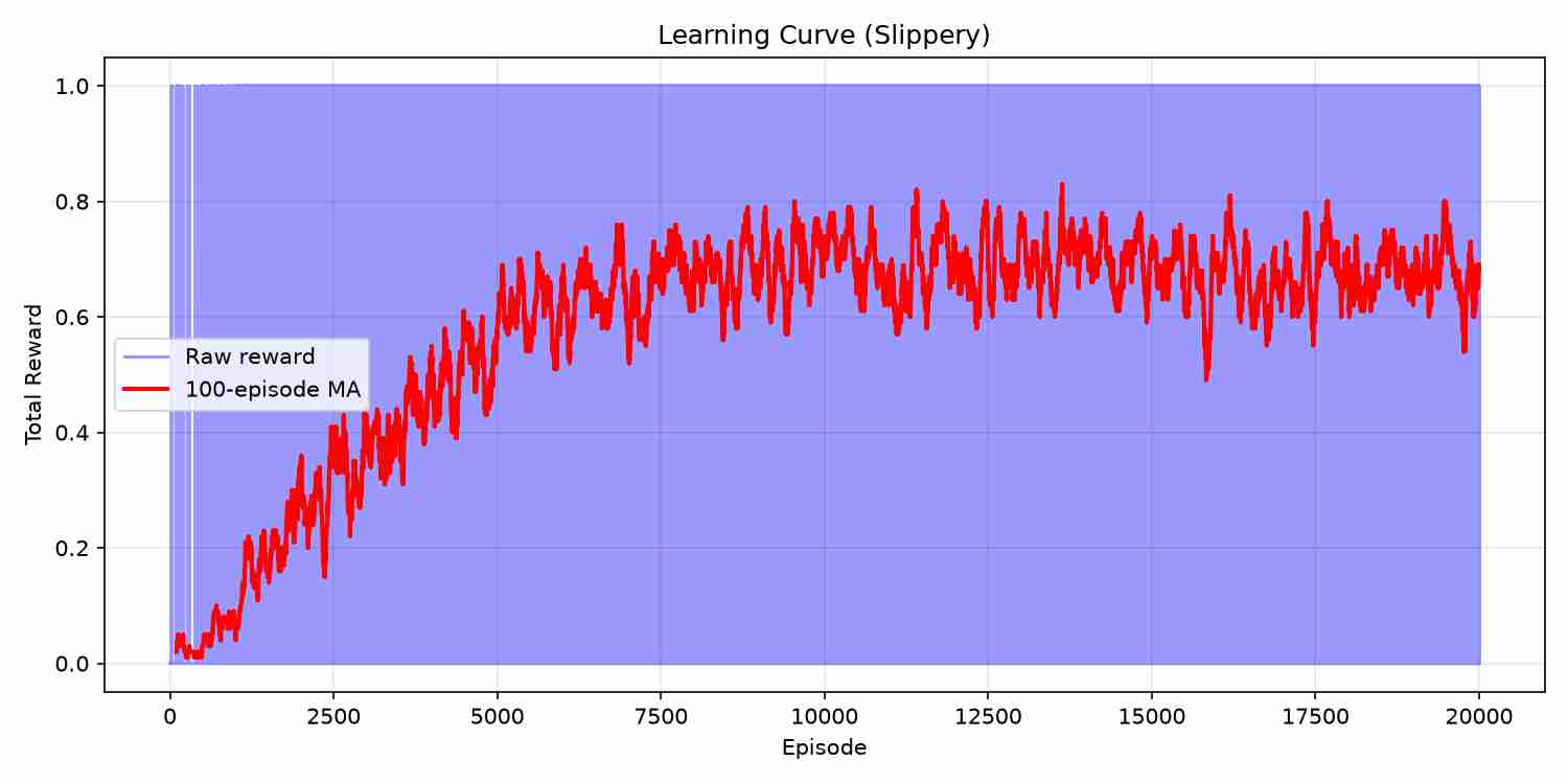
Fig. 3 shows the learning curve for the slippery environment. The raw rewards (blue, transparent) are noisy because the agent's performance varies significantly from episode to episode due to the stochastic nature of the environment. However, the 100‑episode moving average (red) reveals a clear upward trend: the agent starts with very low rewards (near 0, meaning it rarely reaches the goal), and gradually improves over the course of 20,000 episodes. The moving average plateaus around episode 10,000, indicating that the agent has converged to a stable policy. The reward metric in Frozen Lake is simply the total reward per episode (0 or 1), so the moving average essentially tracks the success rate. This plateau around 0.75‑0.80 confirms that the agent has learned a policy that succeeds approximately 75‑80% of the time, which is the best achievable given the stochasticity. The slow, gradual improvement reflects the challenge of learning in a stochastic environment: the agent must average over many random outcomes to accurately estimate the Q‑values.
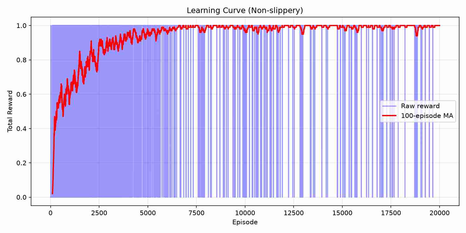
Fig. 4 shows the learning curve for the non‑slippery environment. In stark contrast to the slippery case, the non‑slippery agent learns extremely rapidly. The moving average (red) rises from 0 to 1.0 within approximately 1,500 episodes, after which it remains flat at 1.0. This rapid convergence is expected because the environment is deterministic: once the agent discovers the correct sequence of actions (which it can do through systematic exploration), it can replay that sequence flawlessly every time. The raw rewards (blue) are less noisy than in the slippery case because the outcomes are deterministic. The sharp transition from low to high performance demonstrates that Q‑learning is highly effective for deterministic environments where the optimal policy is a fixed sequence of actions.
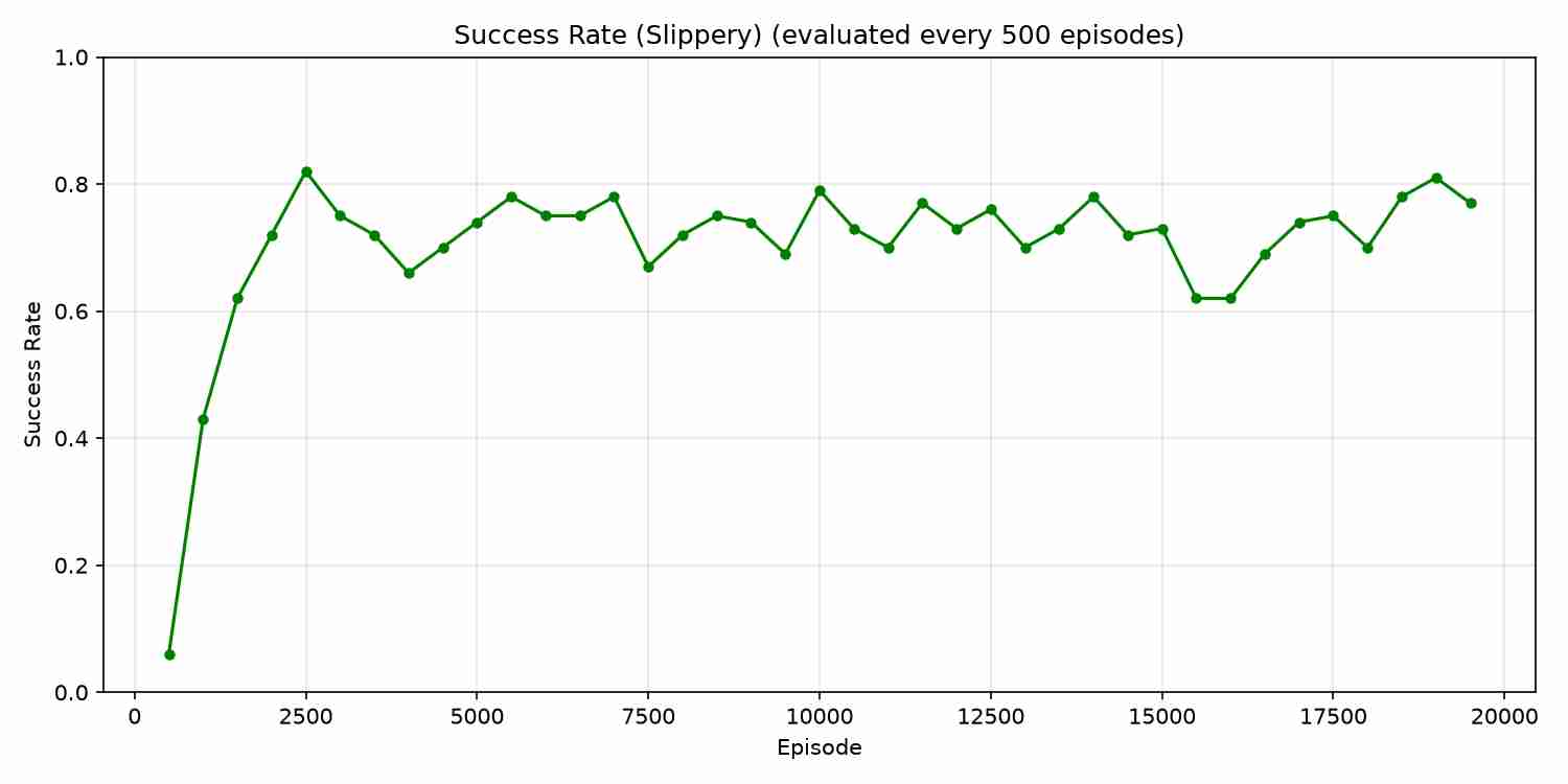
Fig. 5 provides a more detailed view of the learning progress in the slippery environment, showing the success rate at regular evaluation intervals. Each data point represents the agent's performance over 100 test episodes (with exploration disabled) evaluated every 500 training episodes. The curve shows a clear learning trajectory: from 0% success at episode 0, rising gradually through the middle episodes, and finally plateauing at approximately 78% after 10,000 episodes. This gradual improvement reflects the agent's increasing ability to navigate the stochastic environment. The plateau is particularly informative: it indicates that the agent has reached the maximum achievable performance given the environment's inherent randomness. This "success rate ceiling" is not a limitation of Q‑learning but a fundamental property of the problem – even a perfect policy will sometimes fail due to the 1/3 probability of slipping. The steady rise of the curve also demonstrates that Q‑learning effectively handles the temporal credit‑assignment problem: the agent learns to credit actions that led to success many steps later, gradually building a robust policy. The evaluation interval of 500 episodes provides a clear picture of the learning trajectory without excessive noise.
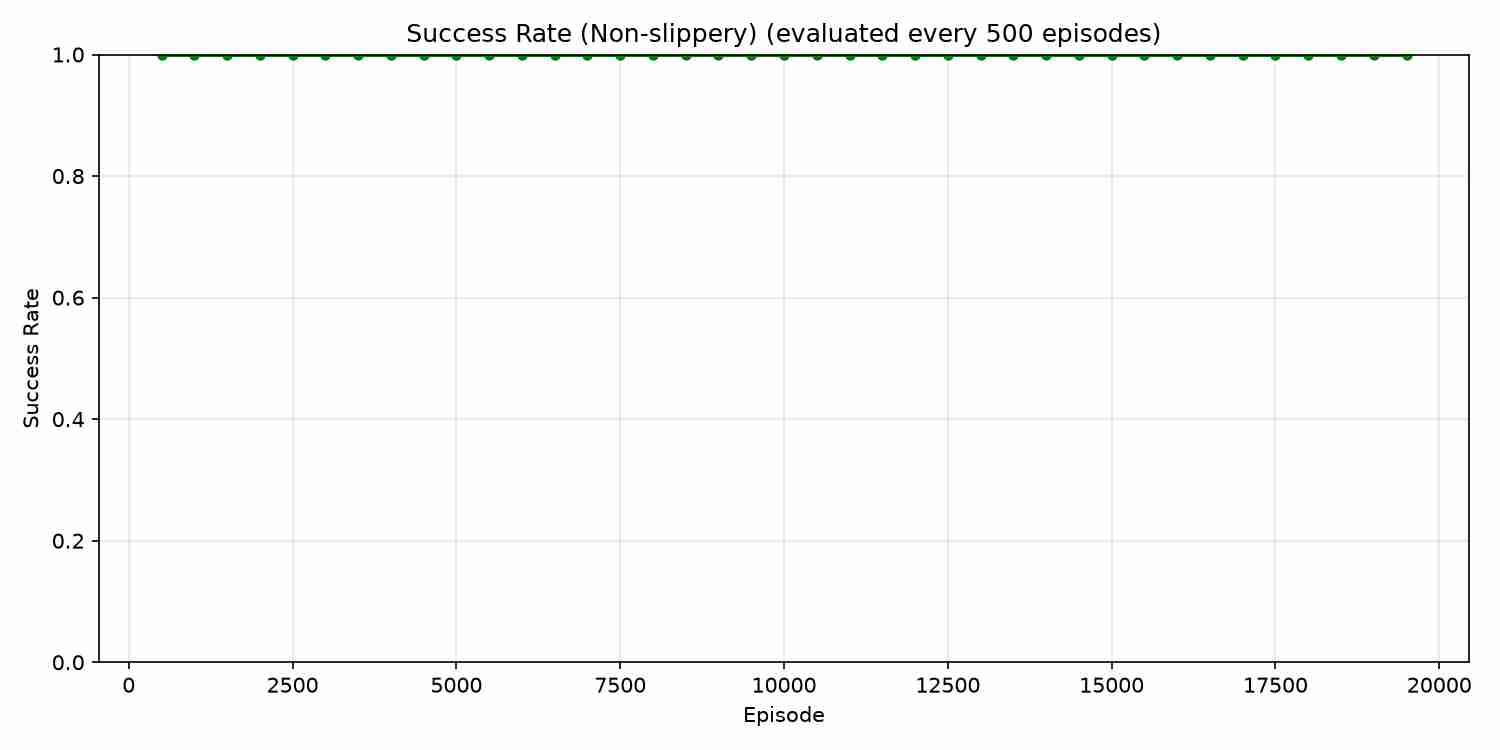
Fig. 6 shows the success rate trajectory for the non‑slippery environment. The success rate rises from 0% to 100% within approximately 1,500 episodes, after which it remains at 100% for the remainder of training. The rapid rise and perfect plateau confirm that the deterministic environment is easily solvable by Q‑learning. The evaluation points every 500 episodes show a clear step‑like improvement: the agent transitions from random exploration to successful exploitation very quickly. This contrasts sharply with the gradual, noisy improvement seen in the slippery environment (Fig. 5), highlighting the profound impact of stochasticity on learning dynamics.
Visualising the Learned Q‑Tables and Policies
The following figures provide deeper insights into what the agent has learned after training on each environment. The Q‑table heatmaps visualise the internal Q‑values, while the policy grids show the greedy actions.
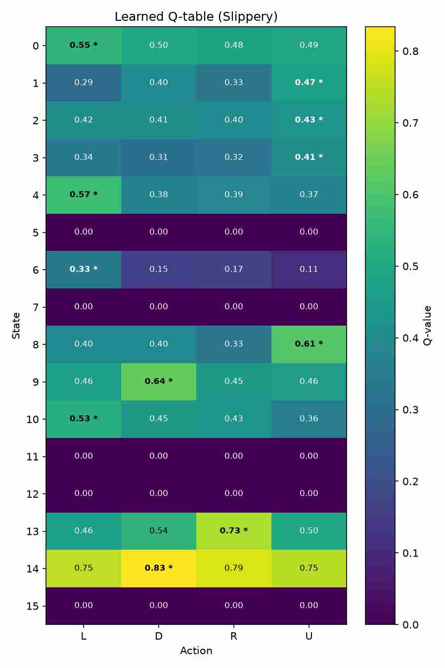
Fig. 7 provides a detailed view into the agent's internal knowledge for the slippery environment. Each row corresponds to one of the 16 states (numbered 0 to 15, matching the grid layout), and each column corresponds to one of the four actions (L = left, D = down, R = right, U = up). The colour intensity reflects the Q‑value: lighter cells represent lower values, while darker cells represent higher values. The greedy action (the action with the highest Q‑value) is marked with an asterisk. Grey cells indicate terminal states (holes and the goal), where the Q‑values are zero because the episode ends immediately upon entering them. Several important patterns emerge from this heatmap. First, states that are adjacent to holes (e.g., states 1, 4, 6, 8, 9) show lower Q‑values overall because the agent has learned that these states are risky – an action that moves toward a hole has a high probability of failure. Second, the Q‑values generally increase as the agent gets closer to the goal (state 15). For instance, state 10 (middle of the bottom row) has high Q‑values for actions that move right (R) and down (D). Third, the agent has learned to avoid actions that move away from the goal: in state 9, the Q‑value for moving up (U) is lower than for moving right (R) or down (D). This heatmap reveals that Q‑learning has successfully internalised the geometry of the grid and the stochastic transition probabilities. A supervised learning model, in contrast, would only see discrete state‑action labels without this rich value information.
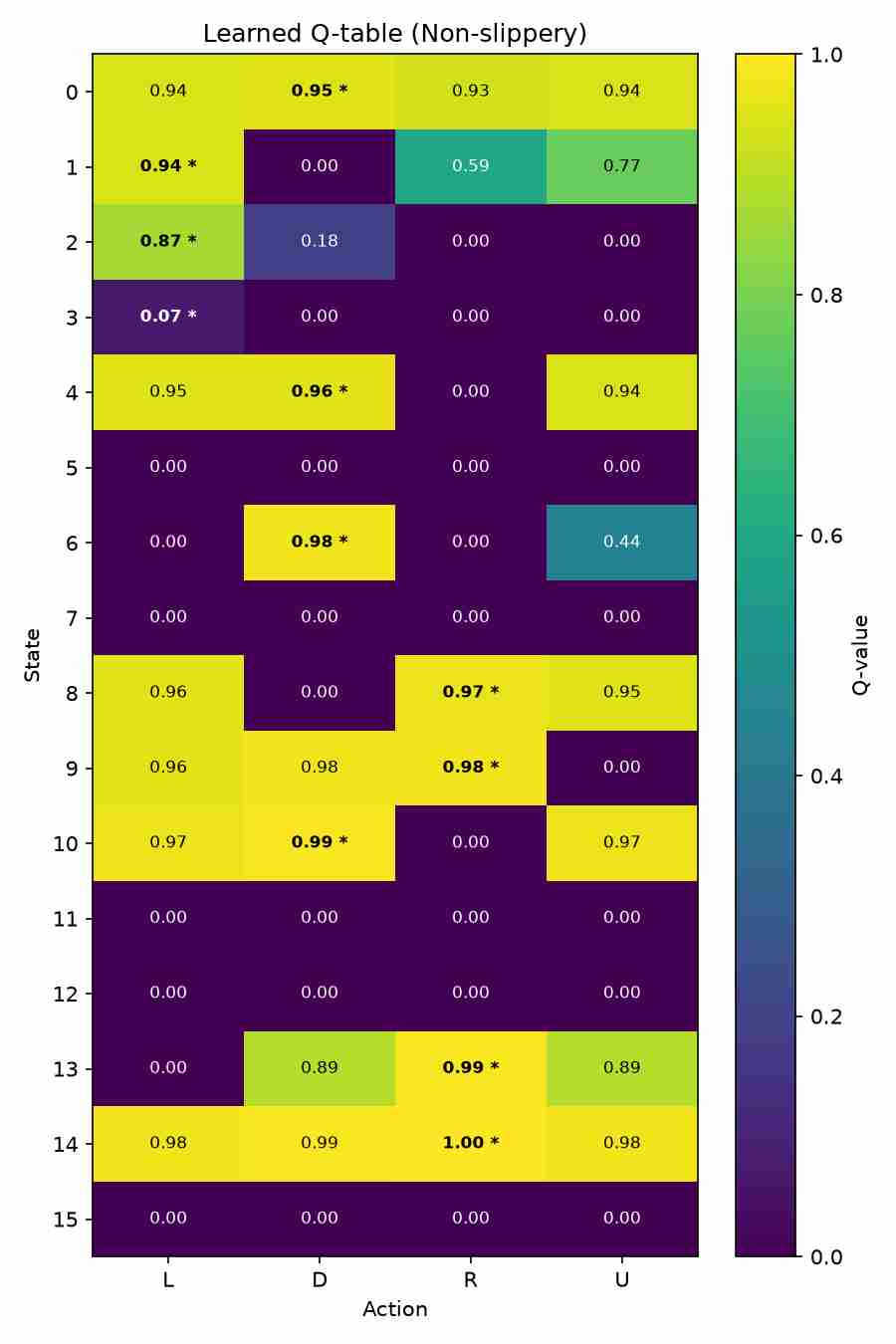
Fig. 8 shows the Q‑table heatmap for the non‑slippery environment. The Q‑values are much higher overall compared to the slippery environment, with many values close to 1.0. This reflects the deterministic nature of the environment: once the agent has learned the correct path, it can reach the goal with 100% certainty, so the expected return from any state on the optimal path is 1.0 (the discount factor γ = 0.99 accounts for the slight reduction). The greedy actions (marked with asterisks) form a clear, unambiguous path from the start to the goal. Terminal states (holes and the goal) have zero Q‑values. The Q‑table for the non‑slippery environment is significantly simpler and more regular than the slippery version, reflecting the absence of uncertainty. The agent has learned a deterministic policy that guarantees success, which is evident from the clean structure of the Q‑table.
Fig. 9 visualises the final greedy policy derived from the Q‑table for the non‑slippery environment. The policy is shown as a 4×4 grid where each cell contains an arrow indicating the best action for that state. The agent has successfully learned a path from the start (top‑left) to the goal (bottom‑right) while navigating around the holes (marked with ✕). The policy respects the geometry of the environment: it moves right and down when possible, avoiding the holes at states 5, 7, and 11. This is exactly the optimal policy one would expect for the non‑slippery version. For the slippery version, the greedy policy would be identical in expectation, but the agent's actual performance would be lower due to the stochastic slips. The policy visualisation confirms that Q‑learning has successfully solved the problem – it has found the correct sequence of actions that leads to the goal without falling into holes.
The visualisations above provide a complete picture of the Frozen Lake problem and the solution learned by Q‑learning. Fig. 2 shows the layout of the environment. Figs. 3 and 4 demonstrate the learning progress for the slippery and non‑slippery environments respectively. Figs. 5 and 6 show the success rate evolution. Figs. 7 and 8 reveal the internal Q‑values for each environment. Fig. 9 visualises the final greedy policy, which is a clean path through the safe tiles.
In summary, Frozen Lake demonstrates the power of RL to handle both deterministic and stochastic environments, to learn from sparse rewards, and to discover policies that are robust to uncertainty. It is a perfect didactic example because it is simple enough to be solved quickly on a laptop, yet rich enough to expose all the key challenges of reinforcement learning.
Key Takeaways
- Reinforcement learning is the computational framework for sequential decision‑making under uncertainty, where an agent learns a policy by interacting with an environment and receiving scalar rewards.
- RL is distinguished from supervised and unsupervised learning by its focus on delayed, sequential feedback, the exploration‑exploitation dilemma, and the temporal credit‑assignment problem.
- The agent–environment loop is the universal architectural pattern; policies, value functions, and (optionally) models are the functional components that enable learning.
- RL algorithms can be classified along several key axes: model‑based vs. model‑free, value‑based vs. policy‑based vs. actor‑critic, on‑policy vs. off‑policy, and tabular vs. deep. Each category has distinct trade‑offs in sample efficiency, stability, and applicability to discrete versus continuous action spaces.
- RL has diverse applications, from robotics and game playing to finance, healthcare, and LLM alignment, wherever decisions have long‑term consequences.
- The Frozen Lake problem is a compelling case study because it is intractable for classification or regression due to non‑deterministic optimal actions, sparse rewards, and the absence of labelled data. The environment's stochasticity (in the slippery version) adds an extra layer of difficulty, requiring the agent to learn a policy that maximises expected return.
- Q‑learning (a model‑free, value‑based, off‑policy algorithm) offers a straightforward yet powerful solution: it learns an action‑value function via temporal‑difference updates, propagates reward information backward through time, and discovers robust strategies even under stochastic transitions.
- With a sufficiently large number of episodes, Q‑learning solves both the non‑slippery and slippery versions, demonstrating the core RL principles in action. The dual‑environment pipeline shows how the same algorithm performs on deterministic versus stochastic problems.
Designing Effective Reward Functions in Reinforcement Learning
The reward function is arguably the most critical design decision in any reinforcement learning system. It defines the objective that the agent will optimise, and its design directly determines what behaviour the agent learns. In the Frozen Lake example, the reward function is deliberately simple: +1 for reaching the goal, 0 for all other transitions (including falling into holes). This sparse reward design forces the agent to explore extensively and learn to credit actions that lead to success, even though the positive feedback only arrives at the very end of a successful episode. While sparse rewards are elegant and align perfectly with the problem's objective, they can make learning extremely slow because the agent receives no guidance about which actions are "good" or "bad" along the way. In more complex environments, practitioners often employ reward shaping – adding intermediate rewards that guide the agent toward desirable behaviour. For example, in a navigation task, one might add a negative reward proportional to distance from the goal at each step, or a positive reward for making progress. However, reward shaping must be done with great care: poorly designed shaped rewards can incentivise unintended behaviours (a phenomenon known as "reward hacking" or "specification gaming"), where the agent exploits the reward structure in ways that do not align with the true objective. A classic example is a cleaning robot that learns to repeatedly drop and pick up dust to maximise a "dust collected" counter without actually cleaning the room.
Several key principles guide the design of effective reward functions in RL. First, the reward should be aligned with the true objective – it should accurately reflect what we want the agent to achieve, not just what is easy to measure. If the objective is to reach a goal, the reward should be positive for reaching the goal and perhaps negative for time spent, so the agent learns to be efficient. Second, rewards should be dense enough to provide useful learning signals but sparse enough to avoid overfitting to intermediate proxies. A common technique is to combine a sparse terminal reward with a small negative reward per step (a "time penalty") to encourage faster solutions. In Frozen Lake, we used +1 for the goal and 0 otherwise, but one could add -0.01 per step to encourage shorter paths. Third, rewards should be Markovian – they should depend only on the current state and action (and perhaps the next state), not on the entire history. This ensures that the MDP formulation remains valid and that the agent can learn optimal policies without maintaining a memory of past events. Fourth, rewards should be bounded to prevent instability in value estimates – unbounded rewards can cause values to grow without bound, making learning unstable. Finally, reward scaling matters: if rewards are too large or too small, they can affect the learning rate and convergence properties. In practice, it is common to scale rewards to be in a reasonable range (e.g., between -1 and 1) to work well with standard hyperparameters.
A powerful extension of basic reward design is reward shaping using potential-based functions. Ng et al. (1999) introduced a formalism for reward shaping that preserves optimality: adding a potential-based shaping reward F(s, a, s') = γ Φ(s') - Φ(s) to the original reward function does not change the optimal policy. This is known as the "potential-based reward shaping" theorem, and it provides a principled way to guide the agent with domain knowledge without altering the optimal policy. For example, in a grid-world, the potential function Φ(s) could be the negative distance to the goal, providing a reward signal that encourages the agent to move closer to the goal at each step. This can dramatically speed up learning in sparse-reward environments while guaranteeing that the agent will still converge to the optimal policy (provided the original reward function is optimal). In more complex domains like robotics, reward functions are often designed through iterative experimentation: define an initial reward function, train the agent, observe its behaviour, and refine the rewards to eliminate undesirable side-effects. This iterative process is sometimes called "reward engineering" and is an essential skill for deploying RL in real-world applications. Ultimately, a well-designed reward function encodes the designer's intent and is the bridge between the problem's objective and the agent's learning process – making it one of the most important, and challenging, aspects of applying reinforcement learning.
The complete, runnable code for every figure above lives in the companion repository under src/. The repository includes scripts to train and evaluate the agent on both deterministic and stochastic versions of Frozen Lake, and to generate the visualisations shown here.
Resources
- [1] Sutton, R. S., & Barto, A. G. — Reinforcement Learning: An Introduction, MIT Press, 2018. incompleteideas.net/book/
- [2] Gymnasium — FrozenLake-v1 Environment, 2023. gymnasium.farama.org/...
- [3] Arulkumaran, K., et al. — A Brief Survey of Deep Reinforcement Learning, IEEE Signal Processing Magazine, 2017. arXiv:1708.05866
- [4] Mnih, V., et al. — Human‑level control through deep reinforcement learning, Nature, 2015. Nature 518, 529–533
- [5] Schulman, J., et al. — Proximal Policy Optimization Algorithms, arXiv, 2017. arXiv:1707.06347
- [6] Brockman, G., et al. — OpenAI Gym, arXiv, 2016. arXiv:1606.01540
- [7] Haarnoja, T., et al. — Soft Actor‑Critic: Off‑Policy Maximum Entropy Deep Reinforcement Learning, ICML, 2018. arXiv:1801.01290
- [8] Ng, A. Y., et al. — Policy Invariance under Reward Transformations: Theory and Application to Reward Shaping, ICML, 1999. ICML 1999