Can a plain stack of convolutions and pooling, with no skip connections and no fancy upsampling, learn to segment a human from the background? It turns out that even a straightforward CNN can produce a coarse mask directly from a larger image. This article walks through training such a network on the LV‑MHP‑v1 multi‑human parsing dataset, using only Conv2d + ReLU + BatchNorm + MaxPool, and shows that with the right loss function you can get meaningful results even without an encoder‑decoder. We then upgrade the architecture with a pretrained ResNet encoder, add extensive data augmentation, monitor IoU during training, and save checkpoints based on the best validation score.
Code: https://github.com/babak-abad/introduction-to-semantic-segmentation
1. What is Semantic Segmentation?
Semantic segmentation is the task of assigning a class label to every pixel in an image. Unlike image classification, which gives one label for the whole picture, and object detection, which draws bounding boxes around instances, segmentation produces a dense pixel‑wise map that precisely delineates object boundaries. For a human parsing scenario, segmentation answers “which pixels belong to a person” rather than “is there a person in this image” (classification) or “where is the person” as a box (detection).
This dense prediction requires the model to understand both the global context (what objects are present) and the fine local structure (where their edges lie). Convolutional neural networks excel at this because they build hierarchical feature maps that capture textures in shallow layers and object parts in deeper layers. When those feature maps are kept spatially aligned, as in a fully convolutional network, the output naturally becomes a per‑pixel classification map — a segmentation mask.
Semantic segmentation is often contrasted with instance segmentation, where every individual object gets its own mask (e.g., “person 1”, “person 2”), and with panoptic segmentation, which unifies semantic and instance tasks. Here we focus on the simplest form — a single binary label per pixel — because it lets us explore the limits of a minimal architecture without the complications of separating overlapping instances.
Historically, segmentation relied on hand‑crafted features and graphical models such as conditional random fields. The advent of fully convolutional networks (FCNs) in 2015 showed that an end‑to‑end trainable CNN could outperform those classic methods by a wide margin. Since then, the dominant trend has been the encoder–decoder architecture (e.g., U‑Net, DeepLab), where a contracting path captures context and an expanding path recovers fine details through skip connections. This article deliberately deviates from that trend: we ask whether a plain, decoder‑free network can still achieve useful results when the output is allowed to be coarse. The answer, as we shall see, is a clear yes.
2. Why Use Segmentation Instead of Detection?
Detection bounding boxes are sufficient when you only need to count objects or estimate their rough location. Segmentation becomes essential when the exact shape matters. For example, an autonomous vehicle needs to know the precise free‑space boundary on the road—a bounding box around a pedestrian is not enough to decide whether the car can pass safely. Likewise, in medical imaging, measuring tumour volume requires a pixel‑accurate mask, not a rectangle. So whenever the application demands shape analysis, area measurement, or precise contour extraction, segmentation is the right tool.
Consider a self‑driving car approaching a crosswalk. A detection system might correctly localise a pedestrian with a bounding box, but it cannot tell whether the pedestrian’s foot is still on the curb or already on the road. Segmentation provides that sub‑box precision, enabling the planner to make a safer decision. Similarly, in agriculture, segmenting crop rows from weeds allows a precision sprayer to target only the unwanted plants, reducing chemical use by over 90% compared to broadcast spraying.
Medical imaging is another domain where masks are irreplaceable. Radiologists often measure tumour size by drawing a contour on a scan; an automated segmentation system can produce that contour consistently and reproducibly, enabling volumetric analysis over time. A bounding box, by contrast, would include healthy tissue and lead to inaccurate volume estimates. In digital pathology, segmenting individual cells is a prerequisite for counting them and detecting abnormalities — a task detection simply cannot do.
Even in seemingly mundane applications, the shape information carried by a mask is valuable. Photo‑editing software uses segmentation to select objects with a single click. Augmented‑reality systems rely on real‑time segmentation to separate the user from the background and insert virtual objects convincingly. In each case, the price of replacing a mask with a box is a loss of precision that, depending on the safety or usability requirements, may be unacceptable. Understanding these trade‑offs helps us appreciate why investing in segmentation, even at coarse resolution, can be a pragmatic choice for resource‑constrained deployments.
3. The LV‑MHP‑v1 Dataset
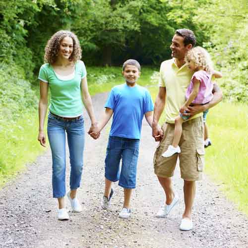
LV‑MHP‑v1 (Large‑scale Multi‑Human Parsing version 1) is a public dataset[1] containing thousands of real‑world images with pixel‑wise annotations for multiple body parts (head, torso, arms, etc.). For this experiment we simplify the task to a single human vs. background binary mask: any pixel that belongs to a person becomes 1, everything else 0. This turns a complex multi‑class problem into a clean two‑class segmentation that a plain CNN can attempt. Fig 1 shows a typical family scene from the dataset, illustrating the variety of poses, occlusions, and lighting conditions the model must handle.
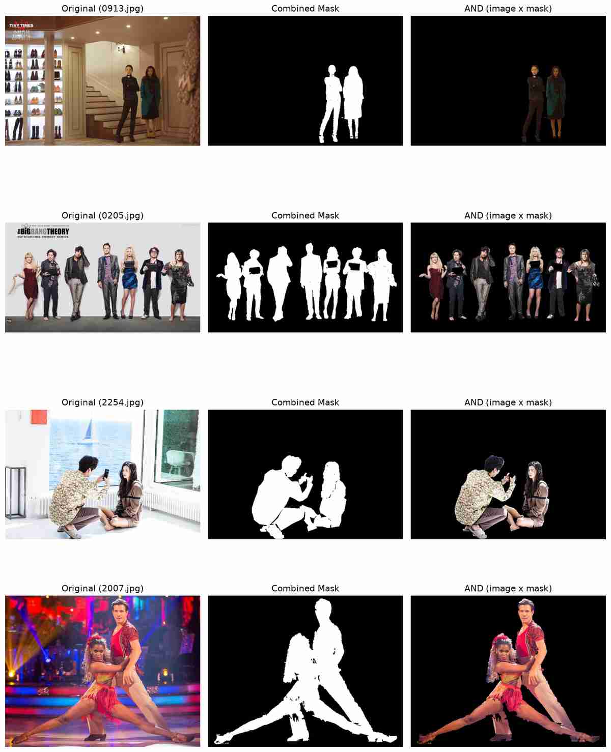
The code below demonstrates how to load an image, merge its per‑person annotations into a single binary mask, and overlay the mask for visual verification. The resulting figure (Fig 2) shows two complete examples, each row consisting of the original photograph, the merged mask, and the pixel‑wise AND (image × mask). The AND operation zeros out the background, leaving only the human regions visible – a quick sanity check that the masks are correctly aligned with the images.
import numpy as np
from PIL import Image
import matplotlib.pyplot as plt

# 1. Load image and mask
image = Image.open("sample.jpg").convert("RGB")
mask_raw = Image.open("sample_mask.png")          # single-channel label image

# 2. Convert to binary: human pixels = 1, background = 0
mask_np = np.array(mask_raw)
binary_mask = (mask_np > 0).astype(np.uint8)     # any non-zero label -> human

# 3. Overlay
plt.figure(figsize=(12,5))
plt.subplot(1,2,1); plt.imshow(image); plt.title("Image")
plt.subplot(1,2,2); plt.imshow(binary_mask, cmap="gray"); plt.title("Binary Mask")
plt.show()
Line 1 imports the required libraries. Lines 4–5 load the original photograph and its annotation mask with Pillow. Line 9 turns the raw label map (where different integer values denote body parts) into a binary array—any pixel whose label is greater than zero becomes 1 (human), otherwise 0 (background). Finally, lines 12–15 display the image and the resulting binary mask side‑by‑side. In the production code, this procedure is repeated for every sample and the multi‑person masks are merged via np.maximum to form a single human‑vs‑background label.
4. Project File Structure
Before diving into the code, here is the layout of the companion repository. All tunable parameters live in a single config.py, and the main training entry point is main.py. Every script under src/ handles one well‑defined part of the pipeline, making the project easy to modify and extend.
| File | Role |
|---|---|
| config.py | Centralised settings: data paths, model hyper‑parameters, augmentation knobs, training options. |
| main.py | Entry point: loads data, builds model, runs training loop, saves best checkpoint, generates demos. |
| src/preprocess.py | Aspect‑ratio preserving resize, zero‑padding, mask binarisation and down‑sampling. |
| src/data_utils.py | Scans the dataset folder, pairs images with mask groups, validates file integrity. |
| src/dataset.py | PyTorch Dataset that merges per‑person masks and applies optional training‑time augmentation. |
| src/augment.py | OpenCV‑based geometric/noise demo augments + albumentations‑based stochastic training pipeline (inc. mixup). |
| src/model.py | Two architectures: Simple_CNN (from scratch) and PretrainedEncoderHead (transfer learning). |
| src/losses.py | BCEWithLogitsLoss + soft Dice loss for imbalanced masks. |
| src/metrics.py | IoU and Dice metrics computed from logits (sigmoid + threshold). |
| src/train.py | Training / validation loops with AMP, mixup, and tqdm progress bars. |
| src/mask_demo.py | Pre‑training visualisation: ground‑truth mask grid and augmentation demo. |
| src/predict.py | Post‑training inference: loads best checkpoint, produces prediction grids for held‑out images. |
| src/viz.py | Shared plotting helpers: learning curves, 3‑column mask figures, PNG+JPG twin export. |
4.1 Configuration Parameters (config.py)
Every aspect of the pipeline is governed by a single configuration file. The parameters are grouped by function; only the ones relevant to training and evaluation need to be changed, and all derived values (like MASK_SIZE) update automatically. The table below summarises every constant and its role.
| Constant | Default / example | Description |
|---|---|---|
| Data & Paths | ||
| DATA_ROOT | "E:/Projects/datasets/LV-MHP-v1" | Root folder containing images/ and annotations/ sub‑directories. |
| IMAGE_SIZE | 640 | Square side length after aspect‑ratio preserving resize and zero‑padding. Must be divisible by 2BLOCK_SIZE. |
| BLOCK_SIZE | 3 | Number of Conv‑BN‑ReLU‑MaxPool blocks; determines the output stride. With IMAGE_SIZE=640 this gives MASK_SIZE=80. |
| MASK_SIZE | 80 (auto‑derived) | Coarse mask resolution; computed automatically from IMAGE_SIZE and BLOCK_SIZE to guarantee alignment. |
| WEIGHTS_DIR | "weights" | Directory where checkpoints are saved (created automatically). |
| WEIGHTS_PATH | "weights/simple_cnn_mhp.pth" | Best checkpoint (highest validation metric). Loaded for inference. |
| LAST_WEIGHTS_PATH | "weights/simple_cnn_mhp_last.pth" | Most recent checkpoint (overwritten every epoch); used for resuming or inspection. |
| ASSET_DIR | "asset" | Directory where demo figures and learning curves are stored. |
| Reproducibility | ||
| SEED | 42 | Master seed for train/val split, demo sampling, and augmentation RNGs. |
| Training | ||
| BATCH_SIZE | 16 | Mini‑batch size (reducible on low‑memory GPUs). |
| LEARNING_RATE | 1e‑3 | Adam initial learning rate. |
| NUM_EPOCHS | 250 | Total training epochs; early stopping may end training sooner. |
| VAL_SPLIT | 0.2 | Fraction of the dataset held out for validation (never trained on). |
| PATIENCE | 10 | Early‑stopping patience: stop if the monitored metric doesn’t improve for this many consecutive epochs. Set to 0 to disable. |
| Hardware | ||
| DEVICE | "cuda" if available else "cpu" | Training device; set manually if needed. |
| NUM_WORKERS | 8 | DataLoader worker threads. |
| PIN_MEMORY | False | Enable pin_memory for faster CPU→GPU transfer (set True when using CUDA with plenty of RAM). |
| PERSISTENT_WORKERS | True | Keep worker processes alive between epochs (faster, uses more RAM). |
| Model Architecture | ||
| IN_CHANNELS | 3 | Input channels (3 for RGB). |
| BASE_CHANNELS | 64 | Number of filters in the first convolution block of Simple_CNN; doubles each subsequent block. |
| Transfer Learning | ||
| USE_PRETRAINED_ENCODER | True | When True, uses a pretrained SMP encoder + head; False falls back to Simple_CNN. |
| ENCODER_NAME | "resnet34" | Pretrained encoder backbone name (any valid smp encoder, e.g. "efficientnet-b0"). |
| ENCODER_WEIGHTS | "imagenet" | Pretrained weights to load; "imagenet" or None. |
| HEAD_CHANNELS | 256 | Hidden channels in the convolutional head attached to the encoder. |
| Loss | ||
| DICE_SMOOTH | 1.0 | Laplace smoothing constant for the Dice loss (avoids division by zero). |
| Prediction | ||
| PRED_THRESHOLD | 0.5 | Binarisation threshold applied to sigmoid output during inference. |
| Visualisation | ||
| VIZ_MAX_WIDTH | 1200 | Maximum width (px) for the JPEG twin of any figure. |
| VIZ_JPEG_QUALITY | 20 | JPEG quality for lightweight preview files. |
| VIZ_DPI | 120 | DPI used when saving PNG figures. |
| FIGSIZE_MASK_GRID | (12,4) | Matplotlib figure size (inches) for mask‑demo and augmentation grids. |
| FIGSIZE_LEARNING_CURVE | (8,5) | Figure size for the learning‑curve plot. |
| MASK_DEMO_SAMPLES | 4 | Number of images shown in the ground‑truth mask demo. |
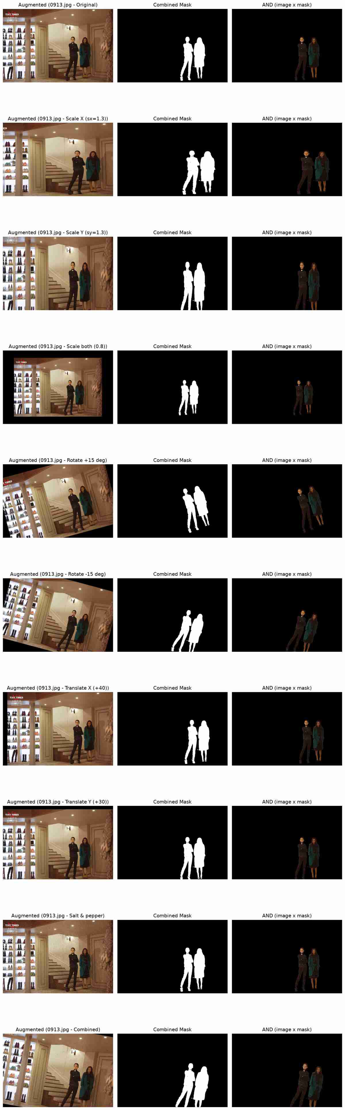
| AUGMENT_DEMO_SAMPLES | 1 | Number of base images run through all 10 augmentation specs. |
| PRED_DEMO_SAMPLES | 4 | Number of validation images shown in the post‑training prediction demo. |
| Static Augmentation Demo | ||
| AUG_SCALE_X, AUG_SCALE_Y | 1.3 | Scale factors for the "Scale X" / "Scale Y" demo specs. |
| AUG_SCALE_BOTH | 0.8 | Uniform scale factor for the "Scale both" spec. |
| AUG_ROTATE_POS / AUG_ROTATE_NEG | 15 / –15 | Rotation angles (degrees) for the positive/negative rotation specs. |
| AUG_TRANSLATE_X, AUG_TRANSLATE_Y | 50 | Pixel translation for the "Translate X" / "Translate Y" specs. |
| AUG_NOISE_AMOUNT | 0.02 | Fraction of pixels corrupted by salt‑and‑pepper noise in the demo. |
| AUG_COMBINED_ROTATE, AUG_COMBINED_SCALE, AUG_COMBINED_NOISE | –10, 1.15, 0.01 | Parameters for the "Combined" spec that applies rotation, scale, and noise together. |
| Training‑time Augmentation | ||
| AUG_TRAIN | True | Master switch for stochastic training augmentation. Set False to disable. |
| AUG_HFLIP / AUG_VFLIP | True | Random horizontal / vertical flips (p=0.5). |
| AUG_ROTATE_LIMIT | 30 | Rotation angle limit (± degrees) for ShiftScaleRotate. |
| AUG_SCALE_LIMIT | 0.2 | Scale jitter limit (± 20%) for ShiftScaleRotate. |
| AUG_TRANSLATE_LIMIT | 0.05 | Translation limit as a fraction of image width/height (± 5%). |
| AUG_BRIGHTNESS_LIMIT, AUG_CONTRAST_LIMIT | 0.2 | Brightness/contrast jitter limits for RandomBrightnessContrast. |
| AUG_HUE_LIMIT, AUG_SATURATION_LIMIT | 10, 20 | Hue / saturation shift limits for HueSaturationValue. |
| AUG_BLUR_PROB | 0.2 | Probability of applying Gaussian blur. |
| AUG_BLUR_LIMIT | 5 | Maximum kernel size for Gaussian blur (must be odd). |
| AUG_CUTOUT_PROB | 0.3 | Probability of applying CoarseDropout (random erasing) to the image. |
| AUG_CUTOUT_HOLES | 4 | Number of cutout rectangles per image. |
| AUG_CUTOUT_HOLE_RATIO | 0.1 | Fraction of image width/height for each cutout rectangle. |
| AUG_MIXUP | True | Enable mixup at batch level. |
| AUG_MIXUP_ALPHA | 0.2 | Alpha parameter for the Beta distribution governing the mixup blending ratio. |
| AUG_MIXUP_PROB | 0.5 | Probability of applying mixup to a given batch. |
| Mixed Precision | ||
| USE_AMP | True | Enable Automatic Mixed Precision (CUDA only) – roughly halves activation memory and speeds up training. |
| Metrics & Checkpoint Selection | ||
| METRIC_THRESHOLD | 0.5 | Threshold applied to sigmoid probabilities when computing IoU and Dice. |
| SAVE_BEST_BY | "iou" | Metric used to choose the best checkpoint and trigger early stopping. Options: "iou", "dice", or "loss". |
With this exhaustive control panel, you can quickly switch between the from‑scratch network and the pretrained encoder, toggle every augmentation, adjust the input size and depth, and decide which metric drives model selection. The rest of the pipeline simply imports config and trusts it for all hyper‑parameters, making experiments fully reproducible with a single file.
5. Data Preprocessing Pipeline
Because LV‑MHP‑v1 images come in varying sizes, we first normalise them to a consistent input dimension. We choose 640×640 as the canonical size: each image is resized so that its longer side fits exactly 640 pixels while preserving the aspect ratio, and the remaining empty area is filled with zero‑padding. The mask undergoes the same geometric transform and is then down‑sampled to the target output size of 80×80 (when BLOCK_SIZE = 3). The exact mask size is derived automatically by compute_output_size to prevent any mismatch between the model output and the ground‑truth labels.
# src/preprocess.py
import cv2
import numpy as np
import torch
import config

IMAGE_SIZE = config.IMAGE_SIZE
MASK_SIZE = config.MASK_SIZE

def resize_with_pad(img_np, target_size=IMAGE_SIZE, is_mask=False):
    h, w = img_np.shape[:2]
    scale = target_size / max(w, h)
    new_w, new_h = int(w * scale), int(h * scale)
    interp = cv2.INTER_NEAREST if is_mask else cv2.INTER_LINEAR
    resized = cv2.resize(img_np, (new_w, new_h), interpolation=interp)

    pad_h = target_size - new_h
    pad_w = target_size - new_w
    top, left = pad_h // 2, pad_w // 2

    if img_np.ndim == 2:
        canvas = np.zeros((target_size, target_size), dtype=img_np.dtype)
    else:
        canvas = np.zeros((target_size, target_size, img_np.shape[2]), dtype=img_np.dtype)
    canvas[top:top + new_h, left:left + new_w] = resized
    return canvas

def image_transform(img_np):
    if img_np.ndim == 2:
        img_np = cv2.cvtColor(img_np, cv2.COLOR_GRAY2RGB)
    else:
        img_np = cv2.cvtColor(img_np, cv2.COLOR_BGR2RGB)
    img_np = resize_with_pad(img_np, target_size=IMAGE_SIZE, is_mask=False)
    tensor = torch.from_numpy(np.ascontiguousarray(img_np)).permute(2, 0, 1).float() / 255.0
    return tensor

def mask_transform(mask_np):
    mask_np = resize_with_pad(mask_np, target_size=IMAGE_SIZE, is_mask=True)
    binary = (mask_np > 0).astype(np.float32)
    mask_tensor = torch.from_numpy(binary).unsqueeze(0)
    mask_tensor = torch.nn.functional.interpolate(
        mask_tensor.unsqueeze(0), size=(MASK_SIZE, MASK_SIZE),
        mode='nearest'
    ).squeeze(0)
    return mask_tensor
Line 1 imports OpenCV. resize_with_pad (line 10) scales the image, preserving aspect ratio; padding is centre‑aligned (lines 17‑21). image_transform converts BGR to RGB and normalises to [0,1]. mask_transform binarises the mask and downsamples to MASK_SIZE with nearest‑neighbour interpolation, keeping the hard 0/1 values.
6. Data Loading and Augmentation
The dataset module (src/dataset.py) reads images with OpenCV and merges per‑person mask annotations into one binary mask via pixel‑wise union. A training‑only augmentation function, passed through augment_fn, transforms the raw numpy arrays before resizing, so image and mask always stay aligned.
6.1 Stochastic Augmentation (albumentations)
The training‑time augmentation pipeline (src/augment.py) uses albumentations for fast, mask‑aware transforms. The default settings include:
- Horizontal & vertical flips (p=0.5 each)
- ShiftScaleRotate: rotation ±30°, scale ±20%, translation ±5%
- Brightness/contrast jitter (±0.2), hue/saturation shifts
- Gaussian blur (p=0.2)
- Cutout / CoarseDropout (four rectangles, p=0.3)
At batch level, mixup blends two images and their soft masks with λ ~ Beta(0.2,0.2) (probability 0.5). Because both loss functions accept float targets, mixup integrates seamlessly.
6.2 Augmentation Code Walkthrough
The actual code that implements these transforms is in src/augment.py. The key functions are _build_train_pipeline, which constructs the albumentations composition from the configuration constants, and random_train_augment, which applies it to a single image–mask pair before they are resized by the preprocessing pipeline. The pipeline is built once (cached) and reused for every training sample, ensuring fast, deterministic behaviour per worker.
def _build_train_pipeline():
    import albumentations as A

    geo = []
    if config.AUG_HFLIP:
        geo.append(A.HorizontalFlip(p=0.5))
    if config.AUG_VFLIP:
        geo.append(A.VerticalFlip(p=0.5))
    geo.append(A.ShiftScaleRotate(
        shift_limit=config.AUG_TRANSLATE_LIMIT,
        scale_limit=config.AUG_SCALE_LIMIT,
        rotate_limit=config.AUG_ROTATE_LIMIT,
        border_mode=cv2.BORDER_CONSTANT, value=0, mask_value=0,
        p=0.9,
    ))

    photo = []
    photo.append(A.RandomBrightnessContrast(
        brightness_limit=config.AUG_BRIGHTNESS_LIMIT,
        contrast_limit=config.AUG_CONTRAST_LIMIT,
        p=0.5,
    ))
    photo.append(A.HueSaturationValue(
        hue_shift_limit=config.AUG_HUE_LIMIT,
        sat_shift_limit=config.AUG_SATURATION_LIMIT,
        val_shift_limit=0,
        p=0.5,
    ))
    photo.append(A.GaussianBlur(
        blur_limit=(3, config.AUG_BLUR_LIMIT),
        p=config.AUG_BLUR_PROB,
    ))
    photo.append(A.CoarseDropout(
        num_holes_range=(config.AUG_CUTOUT_HOLES, config.AUG_CUTOUT_HOLES),
        hole_height_range=(config.AUG_CUTOUT_HOLE_RATIO, config.AUG_CUTOUT_HOLE_RATIO),
        hole_width_range=(config.AUG_CUTOUT_HOLE_RATIO, config.AUG_CUTOUT_HOLE_RATIO),
        fill=0, fill_mask=None,
        p=config.AUG_CUTOUT_PROB,
    ))

    return A.Compose(geo + photo, p=1.0)


_TRAIN_PIPELINE = None

def random_train_augment(img, mask, rng=None):
    global _TRAIN_PIPELINE
    if _TRAIN_PIPELINE is None:
        _TRAIN_PIPELINE = _build_train_pipeline()

    out = _TRAIN_PIPELINE(image=img, mask=mask)
    return out["image"], out["mask"]
Lines 1‑14 build the geometric transform list. If AUG_HFLIP is true (line 5), a HorizontalFlip with probability 0.5 is added; similarly for vertical flips (line 8). The core affine augmentation ShiftScaleRotate (line 9) simultaneously applies translation, scaling, and rotation, with limits taken from the config. The border_mode is set to constant zero filling, and mask_value=0 ensures that the mask border is also filled with background. This transform runs with probability 0.9, so a small fraction of images pass through un‑altered even when augmentation is enabled—a useful regularisation trick.
Lines 16‑36 construct the photometric and erasing transforms. RandomBrightnessContrast (line 17) and HueSaturationValue (line 22) perturb colour channels independently of the mask. GaussianBlur (line 28) uses a randomly sampled odd kernel size up to AUG_BLUR_LIMIT; it only affects the image, not the mask. CoarseDropout (line 32) randomly erases rectangular regions from the image only (fill_mask=None), simulating occlusions. The number of holes and their size ratio are driven by config constants.
Line 38 composes the geometric and photometric transforms with an overall probability of 1.0—every training sample will pass through the full composition. Lines 41‑48 implement the lazy‑initialised entry point random_train_augment. The first call builds and caches the pipeline (line 44); subsequent calls reuse it. The function expects raw H×W×3 numpy arrays and returns the augmented image and mask, still as numpy arrays, ready to be processed by image_transform and mask_transform. This design keeps augmentation completely independent of tensor conversion and resizing, guaranteeing that the mask is transformed by exactly the same geometric operations as the image.
7. Network Architecture
Two architectures are available, both producing raw logits of shape (N,1,MASK_SIZE,MASK_SIZE) so that the loss can use the numerically stable BCEWithLogitsLoss. Despite their simplicity, these models are powerful enough for coarse segmentation because they learn to compress the input into a compact, class‑specific feature representation whose spatial resolution exactly matches the desired output mask. In this section we detail the two variants, then explain the design through the lens of receptive fields and contrast our approach with the popular U‑Net style that includes a decoder and skip connections.
7.1 Simple CNN (from scratch)
Simple_CNN chains BLOCK_SIZE blocks of Conv3×3‑BN‑ReLU‑MaxPool2×2. With BLOCK_SIZE=3 and input 640×640, the feature map after three pools is 80×80. A final 1×1 convolution outputs a single logit channel. The number of filters starts at base_channels (64) and doubles after each block (see Fig 3).
7.2 Pretrained Encoder + Head (Transfer Learning)
Training a segmentation model from scratch needs many annotated samples. Transfer learning re‑uses an encoder pretrained on ImageNet. PretrainedEncoderHead wraps a backbone (e.g., resnet34) from segmentation_models_pytorch and attaches a small Conv‑BN‑ReLU head. The encoder depth equals BLOCK_SIZE (3), so the output stride matches MASK_SIZE. ImageNet normalisation is folded inside the forward pass, so the model still accepts [0,1] tensors.
# src/model.py (excerpt)
class PretrainedEncoderHead(nn.Module):
    def __init__(self, ...):
        self.encoder = smp.encoders.get_encoder(
            encoder_name, in_channels=in_channels,
            depth=self.depth, weights=encoder_weights)
        enc_ch = self.encoder.out_channels[-1]
        self.head = nn.Sequential(
            nn.Conv2d(enc_ch, head_channels, 3, padding=1),
            nn.BatchNorm2d(head_channels), nn.ReLU(inplace=True),
            nn.Conv2d(head_channels, head_channels, 3, padding=1),
            nn.BatchNorm2d(head_channels), nn.ReLU(inplace=True),
            nn.Conv2d(head_channels, 1, 1),
        )
        # ... ImageNet mean/std buffers ...

    def forward(self, x):
        x = (x - self.norm_mean) / self.norm_std
        feats = self.encoder(x)
        logits = self.head(feats[-1])
        return F.interpolate(logits, size=(self.mask_size, self.mask_size),
                             mode='bilinear', align_corners=False)
Lines 3‑6 instantiate the pretrained encoder using smp.encoders.get_encoder. The depth parameter (set to BLOCK_SIZE) controls how many down‑sampling stages are kept, matching the desired output stride. Lines 7‑14 build the convolutional head: two Conv‑BN‑ReLU blocks with head_channels filters, followed by a 1×1 convolution that collapses to a single logit channel. Line 18 applies ImageNet normalisation (stored as buffers). Line 20 takes the deepest feature map from the encoder and passes it through the head. A defensive bilinear interpolation (line 21) guarantees the output spatial size is exactly MASK_SIZE, correcting any rounding errors from unusual input dimensions or stride mismatches.
7.3 Receptive Fields — The Hidden Context Window
One of the most important yet often overlooked properties of any convolutional network is its receptive field. For a given neuron in the output feature map, the receptive field is the patch of the input image that affects its value. Each convolution and each pooling operation expands this patch according to well‑defined rules, so that deeper layers effectively “see” larger regions of the input. In a network without dilated convolutions, the receptive field grows linearly with the number of layers and multiplicatively with the strides of pooling operations. Understanding this growth is key to appreciating why even a simple down‑sampling network can produce meaningful segmentation masks.
The size of the receptive field after a sequence of layers can be computed recursively. Let rin be the receptive field at the input of a layer, and let jin be the “jump” — the distance in the input image between two adjacent features. For a convolution with kernel size k and stride s, the new receptive field rout and jump jout are
  rout = rin + (k − 1) · jin
  jout = jin · s
Starting from the input layer, where every feature corresponds to a single pixel (r0 = 1, j0 = 1), we can trace the effect of each operation in our Simple_CNN. The following table shows the result for a typical configuration with four Conv‑MaxPool blocks. Each 3×3 convolution (padding = 1, stride = 1) adds (3‑1)×jin to the receptive field without changing the jump. Each 2×2 MaxPool (stride = 2) doubles the jump and contributes a small extra amount to the receptive field from its kernel size.
| Layer | Kernel (k) | Stride (s) | Jump (j) | Receptive Field (r) |
|---|---|---|---|---|
| Input | — | — | 1 | 1 |
| Conv1 (3×3) | 3 | 1 | 1 | 3 |
| MaxPool (2×2) | 2 | 2 | 2 | 4 |
| Conv2 (3×3) | 3 | 1 | 2 | 8 |
| MaxPool (2×2) | 2 | 2 | 4 | 12 |
| Conv3 (3×3) | 3 | 1 | 4 | 20 |
| MaxPool (2×2) | 2 | 2 | 8 | 28 |
| Conv4 (3×3) | 3 | 1 | 8 | 44 |
| MaxPool (2×2) | 2 | 2 | 16 | 60 |
After four down‑sampling stages, each output pixel synthesises information from a 60×60 window in the original 640×640 input. In our actual configuration we use BLOCK_SIZE = 3, which gives a receptive field of approximately 45×45 at the 80×80 output. This window is large enough to capture the local texture and shape of a limb, a torso, or a head, along with sufficient surrounding context to disambiguate foreground from background. However, it is not large enough to see the whole person at once—and that is perfectly acceptable for a coarse 80×80 prediction, because each output pixel needs only local evidence to decide whether it belongs to a person. The network can therefore rely on the statistical regularity of human appearance and the fact that neighbouring pixels often share the same class, without ever needing a global understanding of the entire scene.
The same principle applies to the pretrained encoder variant. A ResNet‑34 with three down‑sampling stages has a comparable receptive field, and the small convolutional head that follows does not alter it substantially. Transfer learning provides a head start because the encoder already knows about edges, textures, and object parts from ImageNet; the head simply re‑purposes that knowledge for human‑vs‑background segmentation at the given output stride. The combination of a well‑sized receptive field and strong pretrained features is what allows this simple architecture to reach IoU scores above 0.85 after only a few hundred epochs.
7.4 Why No Decoder and No Skip Connections?
In semantic segmentation, the term encoder refers to the part of a network that progressively reduces spatial resolution while increasing feature depth—exactly what both Simple_CNN and the pretrained ResNet‑34 do. A decoder, in contrast, is an up‑sampling path that recovers spatial detail from the compressed features, often using transposed convolutions or bilinear interpolation combined with skip connections that bring back fine‑grained information from earlier layers. The classic U‑Net is the canonical example: an encoder–decoder with symmetric skip connections that produces a full‑resolution mask.
Our architectures deliberately omit the decoder and skip connections. The reason is twofold. First, the target output is already at a low resolution—80×80 rather than the original 640×640. The heavy down‑sampling of the encoder naturally discards the high‑frequency details that a decoder would normally restore, but since we never ask for those details, there is no need to reconstruct them. Second, skip connections exist precisely to recover spatial precision that is lost during down‑sampling. When the output is sixteen times smaller in each dimension, the localisation demands are so relaxed that the coarse feature map of the deepest encoder layer already contains enough information to decide whether a pixel is foreground or background. Adding a decoder would merely increase the number of parameters and the risk of overfitting without providing a commensurate gain in accuracy for this specific task.
In effect, we are using the encoder as the entire model, with a tiny projection head acting as a “classification layer” applied densely to every spatial position. This is sometimes called a fully convolutional network with down‑sampling only or an encoder‑only segmentation network. It is not suitable for tasks that require pixel‑perfect boundaries, but it is remarkably efficient for coarse localisation, counting, attention‑prior generation, and any other scenario where a rough silhouette suffices. By studying this minimal design, we gain a clearer understanding of what the encoder alone can achieve, and we establish a solid baseline against which more complex architectures can be measured.
8. Loss Functions and Metrics for Semantic Segmentation
In a typical street‑scene image, the human occupies only a small fraction of the pixels; the vast majority are background. A plain binary cross‑entropy (BCE) loss can become dominated by the easy negative examples, causing the network to predict all‑zeros and ignore the object. The Dice loss, directly derived from the Dice similarity coefficient, bypasses this imbalance by focusing on the overlap between the predicted and ground‑truth masks. Our implementation uses BCEWithLogitsLoss for numerical stability and computes Dice on the sigmoid of logits.
# src/losses.py
import torch.nn.functional as F

def dice_loss(logits, target, smooth=1.0):
    pred = torch.sigmoid(logits)
    pred_flat = pred.contiguous().view(-1)
    target_flat = target.contiguous().view(-1)
    intersection = (pred_flat * target_flat).sum()
    return 1 - (2. * intersection + smooth) / (pred_flat.sum() + target_flat.sum() + smooth)

def combined_loss(logits, target, smooth=1.0):
    bce = F.binary_cross_entropy_with_logits(logits, target)
    dice = dice_loss(logits, target, smooth)
    return bce + dice
The dice_loss function (line 4) flattens sigmoid probabilities, computes intersection, and returns 1 − Dice. combined_loss (line 13) adds BCEWithLogitsLoss to Dice, giving stable gradients for all pixels while aggressively correcting overlap on the foreground.
Numerical example – small 2×2 mask. To see why Dice loss works better under imbalance, consider a tiny 2×2 mask where three pixels are background (0) and one pixel is foreground (1). Suppose an untrained model predicts a constant probability of 0.01 for every pixel (essentially all‑background). The BCE loss averages the four pixel contributions:
LBCE = −¼ [ 3·log(1−0.01) + 1·log(0.01) ] ≈ 1.18
This number seems reasonable, but notice that the three easy background pixels contribute −log(0.99) ≈ 0.01 each, while the single missed foreground pixel contributes −log(0.01) ≈ 4.6. Despite the drastic misprediction on the foreground, the average is diluted by the many correct background predictions. The gradient signal for the foreground is weakened.
Now compute the Dice loss on the same prediction with a smooth constant ε = 1. The intersection sum is 0.01×1 = 0.01; the sum of predictions is 4×0.01 = 0.04; the sum of ground truth is 1. The Dice coefficient is 2·(0.01) / (0.04 + 1) ≈ 0.0192, giving a Dice loss of 1 − 0.0192 = 0.98 (with smoothing the value is similar). This loss is close to 1, strongly penalising the missed foreground pixel regardless of the many correct background predictions. The gradient from Dice loss will be concentrated on the single mispredicted pixel, forcing the network to increase that probability. Combining the two losses gives a total loss of ≈ 1.18 + 0.98 = 2.16, where the Dice component prevents the model from ignoring the rare class.
Numerical example – realistic 64×64 mask. A more realistic scenario is a 64×64 output where the foreground object occupies roughly a 5×5 circle (25 pixels) out of 4096 pixels total—only 0.6% of the mask. Suppose again the network predicts a constant probability of 0.01 everywhere, ignoring the object entirely. The BCE loss, averaged over all 4096 pixels, becomes
LBCE = −(1/4096) [ 4071·log(0.99) + 25·log(0.01) ] ≈ 0.038
This tiny loss gives the illusion that the model is already doing well, because the 4071 correctly predicted background pixels dominate the average. The 25 missed foreground pixels barely raise the value. In contrast, the soft Dice loss (with ε = 1) is
  Intersection = 25 × 0.01 = 0.25
  Σ pred = 4096 × 0.01 = 40.96,   Σ target = 25
  Dice = 2·0.25 / (40.96 + 25) ≈ 0.0076  →  LDice ≈ 0.992
The Dice loss is close to 1, clearly signalling that the object is being completely missed. Because the Dice denominator is dominated by the predicted and true foreground sums, it ignores the massive correct background, forcing the network to care about the small object. This dramatic difference—0.038 vs. 0.992—is why Dice loss (or its combination with BCE) is essential for imbalanced segmentation, and it is especially important in our coarse masks where a human silhouette may still be only a few tens of pixels. Fig 5 visualises a 64×64 mask with a tiny 5×5 foreground block.
8.1 Mathematical Foundations of the Loss Functions
The two loss components used in training—binary cross‑entropy and the Dice loss—each have a distinct mathematical form and gradient behaviour. Understanding these helps explain why their combination is so effective for highly imbalanced segmentation tasks.
Binary Cross‑Entropy (BCE). For a single pixel with true label y ∈ {0,1} and predicted probability p ∈ [0,1], the BCE loss is
LBCE(p, y) = −[ y · log(p) + (1 − y) · log(1 − p) ]
Averaged over all N pixels of an image, the total BCE loss is the mean of these per‑pixel contributions. Because each pixel contributes equally to the sum, a dataset where 95% of pixels are background will cause the network to focus overwhelmingly on background classification. The gradient of BCE with respect to the pre‑activation logit z (where p = σ(z)) is ∂L/∂z = p − y. For an easy background pixel (y=0, p≈0), this gradient is near zero, so the network receives little signal to correct errors on rare foreground pixels.
Dice Loss. The Dice coefficient for two binary masks X (prediction) and Y (ground truth) is
Dice(X, Y) = 2|X ∩ Y| / (|X| + |Y|)
In a soft, probabilistic setting where each pixel i has predicted probability pi and ground truth yi ∈ {0,1}, the soft Dice loss is defined as
LDice = 1 − (2 Σi pi yi + ε) / (Σi pi + Σi yi + ε)
where ε is a smoothing constant (e.g., 1) to avoid division by zero. The numerator emphasises the intersection: it grows when the model assigns high probability to true foreground pixels. The denominator normalises by the total number of predicted and true foreground pixels, making the loss independent of the background size. Consequently, the gradient flow from Dice loss is concentrated on the overlapping region, strongly penalising false negatives and false positives on the object of interest, even when the object occupies only a tiny fraction of the image.
Combined Loss Dynamics. The final loss used is L = LBCE + LDice. BCE ensures that every pixel receives some gradient, stabilising early training and preventing the network from collapsing to an all‑zero output. Dice loss then sharpens the mask by directly optimising the spatial overlap. Empirically, this combination converges faster than either loss alone and produces higher IoU scores on the minority class.
8.2 Evaluation Metrics: Dice and IoU
While the Dice loss is used for training, the actual evaluation of a trained model is done with the Dice coefficient and the Intersection over Union (IoU), also known as the Jaccard index. For binary masks X (predicted) and Y (ground truth), the two metrics are defined as:
  Dice(X, Y)  = 2|X ∩ Y| / (|X| + |Y|)
  IoU(X, Y)   = |X ∩ Y| / |X ∪ Y|    = Dice / (2 − Dice)
Both range from 0 to 1 (higher is better). IoU is always more conservative than Dice; for example, a Dice of 0.8 corresponds to an IoU of approximately 0.67. When evaluating after training, we threshold the sigmoid output at 0.5 to obtain a binary mask and compute the metric on the whole validation set. The metrics module implements these directly from logits, applying sigmoid and thresholding internally:
@torch.no_grad()
def iou_score(logits, target, threshold=0.5, smooth=1e-7):
    pred = (torch.sigmoid(logits) > threshold).float()
    inter = (pred * target).sum(dim=(1,2,3))
    union = (pred + target).clamp(0,1).sum(dim=(1,2,3))
    return (inter + smooth) / (union + smooth)  # mean over batch
The function thresholdes the sigmoid at line 3, computes intersection and union per image, and returns the batch‑average IoU. A similar dice_score uses the same approach. This implementation gives equal weight to every image in the batch, which is appropriate because all masks have been resized to the same MASK_SIZE.
9. Training Loop with PyTorch
The main script (main.py) handles deterministic data splitting, model building, and the training loop. Key features include:
- Training data receives stochastic augmentation; validation stays clean.
- Automatic Mixed Precision (AMP) with gradient scaling on CUDA.
- IoU, Dice, and loss are logged every epoch.
- Checkpoints are saved every epoch (LAST_WEIGHTS_PATH) and the best model (by highest val IoU) is saved separately.
- Early stopping stops training when val IoU does not improve for PATIENCE epochs.
# main.py (excerpt)
model = build_model().to(config.DEVICE)
optimizer = torch.optim.Adam(model.parameters(), lr=config.LEARNING_RATE)
scaler = torch.amp.GradScaler("cuda", enabled=use_amp)

best_metric = -1.0   # maximise IoU
for epoch in range(1, config.NUM_EPOCHS+1):
    train_loss = train_one_epoch(model, train_loader, optimizer, device, scaler)
    val_loss, val_iou, val_dice = validate(model, val_loader, device)

    torch.save(model.state_dict(), config.LAST_WEIGHTS_PATH)
    if val_iou > best_metric:
        best_metric = val_iou
        torch.save(model.state_dict(), config.WEIGHTS_PATH)
        print(f"  -> new best IoU: {val_iou:.4f}")

    if config.PATIENCE and epochs_no_improve >= config.PATIENCE:
        break
The train_one_epoch function (inside src/train.py) applies mixup, forward/backward with AMP, and returns the average training loss. validate computes loss, IoU, and Dice without gradient. The best‑checkpoint logic (lines 8‑11) saves the weights only when validation IoU exceeds all previous values, ensuring the final model is the one that generalises best.
10. Results and Learning Curves
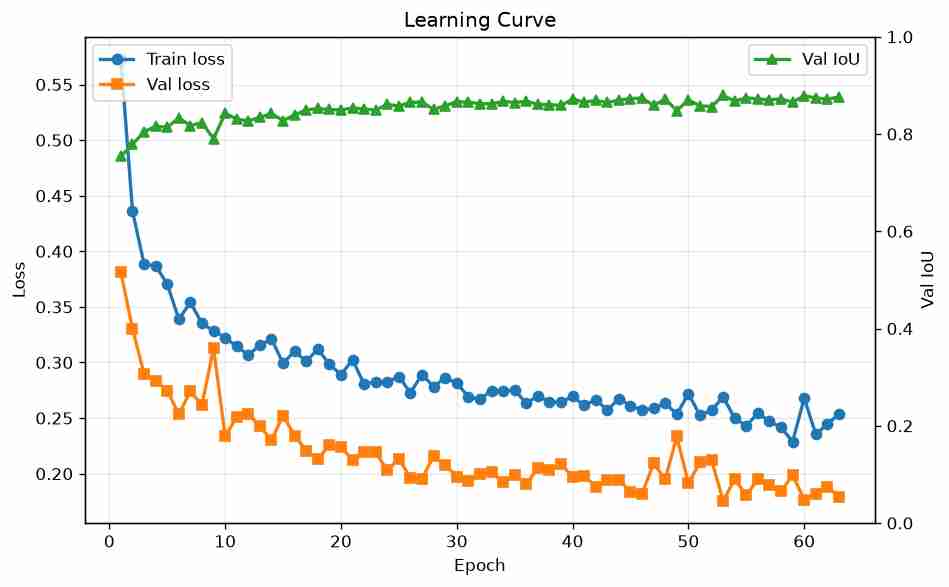
After training, the script automatically generates a learning‑curve plot (Fig 6). The combined BCE+Dice loss steadily decreases, while the validation IoU climbs from near zero to around 0.85–0.90 with the ResNet‑34 encoder. The twin‑axis layout places the train/validation loss on the left axis and the validation IoU on the right axis, making it easy to spot the best epoch for checkpoint saving. Even with the simpler Simple_CNN, the curves demonstrate that a plain down‑sampling network can learn a meaningful coarse mask when paired with suitable augmentation and loss functions.
11. Qualitative Results and Visual Demos
After training, the best checkpoint (by validation IoU) is used for inference. The prediction demo (predict.py) generates a grid of “Original | Predicted Mask | AND” for held‑out validation images (Fig 7). The ground‑truth mask demo (already shown in Fig 2) provides the corresponding reference before training.
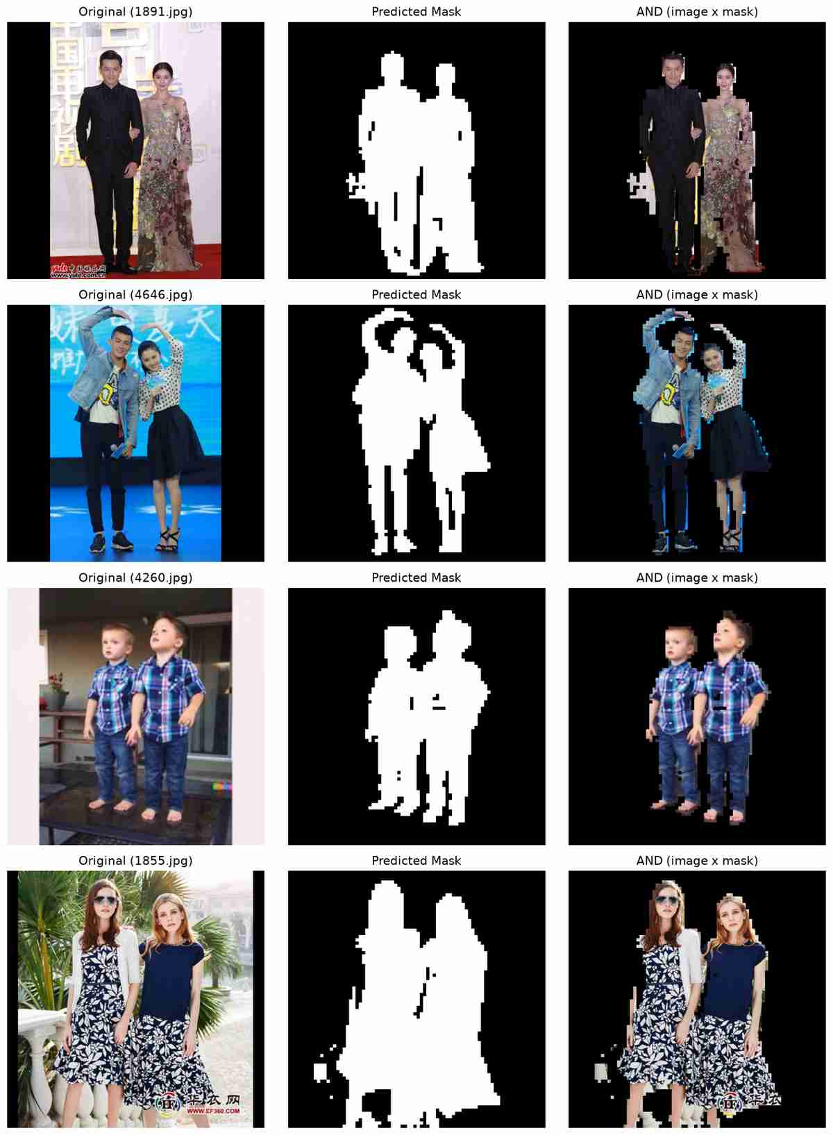
At coarse resolution, the model captures the overall silhouette but misses thin structures like fingers or loose hair. Upsampling the mask to the original image size reveals blocky edges. Nevertheless, for applications such as coarse person location, crowd counting, or as a cheap attention prior, this resolution is often sufficient and comes with the benefit of an extremely simple and fast model.
Key Takeaways
- A plain CNN (or a pretrained encoder) without skip connections can be trained for coarse segmentation when paired with a strong loss and data augmentation.
- Transfer learning with a pretrained ResNet backbone drastically reduces training time and improves results when annotated data is scarce.
- BCEWithLogitsLoss + Dice loss is numerically stable and handles severe class imbalance, as demonstrated by the numerical examples.
- Monitoring validation IoU and using early stopping / checkpoint‑by‑IoU ensures the best model is retained, even when loss briefly fluctuates.
- Extensive, mask‑aware augmentation (including mixup) significantly boosts generalisation without desynchronising image–mask alignment.
- All tunable parameters are centralised in a single config.py file, making experiments reproducible and easy to adjust.
The complete, runnable code for every figure above lives in the companion repository under src/. Full attribution for every dataset and library is in the repository's RESOURCES.md.
Resources
Every asset, dataset, and library cited above — numbered in order of first appearance. Sample assets are used under the license noted for each; the derived images in this article are derivative works of them. Click any bracketed marker such as [1] to jump to its entry.
- [1] LV‑MHP‑v1: A Large‑scale Multi‑Human Parsing Dataset — J. Li et al., Multi‑Human Parsing in the Wild, arXiv 2017. Provided for research use. lv-mhp.github.io
- [2] PyTorch — BSD‑style license. pytorch.org
- [3] segmentation_models_pytorch — MIT license. github.com/qubvel/segmentation_models.pytorch
- [4] albumentations — MIT license. github.com/albumentations-team/albumentations