An Adhoc OCR for License-Plate Character Recognition

In this article we build a small, fully transparent Optical Character Recognition (OCR) engine for the characters of a license plate, and we walk through every stage so you can see exactly what happens to the image. The goal is educational: an adhoc model you can read end to end, not a production system. By the end you will have a pipeline that turns a cropped plate image into a text string, trained without downloading any labelled character dataset - and we will be honest about where it succeeds and where it breaks on real-world plates. The complete source code is on GitHub at github.com/babak-abad/Adhoc_OCR.

1. What is OCR?

Optical Character Recognition (OCR) is the task of converting an image of text - printed or handwritten - into machine-readable characters. Instead of treating a photo of the word HELLO as a grid of pixels, OCR returns the five symbols H, E, L, L, O. A classic OCR system is built from a chain of steps: it cleans the image, separates (segments) the individual glyphs, describes each glyph with a set of numeric features, and finally asks a trained classifier "which character is this?".

2. Where is OCR used?

OCR is one of the most widely deployed computer-vision technologies. Common uses include:

• Document digitisation - scanning books, forms and invoices into searchable text.
• Banking - reading cheques, IBANs and payment slips.
• Data entry automation - extracting fields from passports, ID cards and receipts.
• Accessibility - reading text aloud for visually impaired users.
• Translation apps - recognising text in a photo before translating it.
• Automatic License-Plate Recognition (ALPR) - reading vehicle plates for tolling, parking and access control.

This article focuses on the last one. License-plate recognition is an OCR problem that runs after a separate step has already located the plate inside the full scene. A detector (for example a Haar cascade, YOLO or a contour heuristic) finds the rectangle of the plate and crops it; our OCR then reads the characters inside that crop. In this project we assume the plate has already been detected and we receive the cropped plate as input.

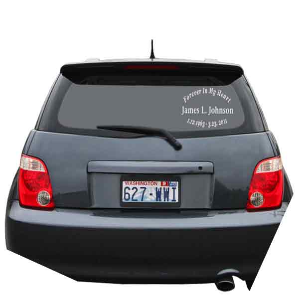
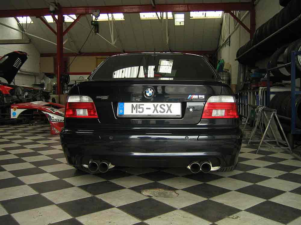
Figure 1. Real scenes from the OpenALPR Benchmark dataset. A detection step must first crop the plate region; the OCR in this article works on that crop.

3. The pipeline at a glance

The recognition path has six stages. Figure 2 shows all of them on a single plate; the rest of the article explains each one.

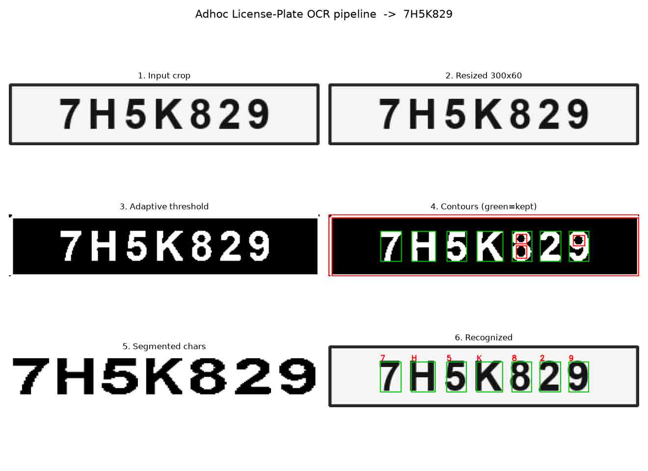
Figure 2. The complete adhoc OCR pipeline, end to end, producing the string 7H5K829.

1. Resize the plate to a canonical size (300 × 60).
2. Adaptive thresholding (binarisation).
3. Find all contours.
4. Remove non-character contours by their geometric properties.
5. Extract features (geometric moments + hue) from each character.
6. Classify each character with an SVM and read them left to right.

4. Stage 1 - Normalise the plate size

Plates arrive at many resolutions. We first resize every crop to a fixed 300 × 60 frame so that all later thresholds and size filters have a predictable scale to work against. The helper is resize_plate in src/preprocess.py.

def resize_plate(image, width=config.PLATE_WIDTH, height=config.PLATE_HEIGHT):
    """Stage 1 - bring every plate to one canonical size."""
    return cv2.resize(image, (width, height), interpolation=cv2.INTER_CUBIC)

In line 1 the function resize_plate is declared; its arguments width and height default to config.PLATE_WIDTH (300) and config.PLATE_HEIGHT (60), so every crop is forced to the same 300 × 60 frame. Line 2 is the docstring naming the stage. In line 3, cv2.resize rescales the image to (width, height), and the cv2.INTER_CUBIC interpolation keeps the up-scaled strokes smooth rather than blocky.

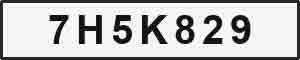
Figure 3. Stage 1 - the plate normalised to 300 × 60.

5. Stage 2 - Adaptive thresholding (and why it is mandatory)

Binarisation turns the grey plate into a black-and-white image so that the characters become solid shapes we can outline. The naive way is a global (static) threshold: pick one brightness value T and call every pixel below it "ink" and every pixel above it "background". This works only when the whole plate is lit evenly - which a real plate almost never is.

In the real world a plate carries a brightness gradient: sunlight on one half, a shadow from the bumper or a mud-guard on the other, headlight glare, or simply the curvature of the plate. With a single global T the dark half of the plate falls entirely below the threshold, so its characters merge into one black blob, while the bright half may wash out completely. No single value can be right everywhere.

Adaptive thresholding solves this by computing a separate threshold for every small neighbourhood (here a 21 × 21 window), so a shadow on one side of the plate no longer destroys the characters on it. Figure 4 makes the difference concrete on a real European plate with a simulated shadow falling across it: both global methods (a fixed cut-off and Otsu's automatic one) lose the S and X on the shadowed right side, while adaptive thresholding still recovers the whole M5-XSX.

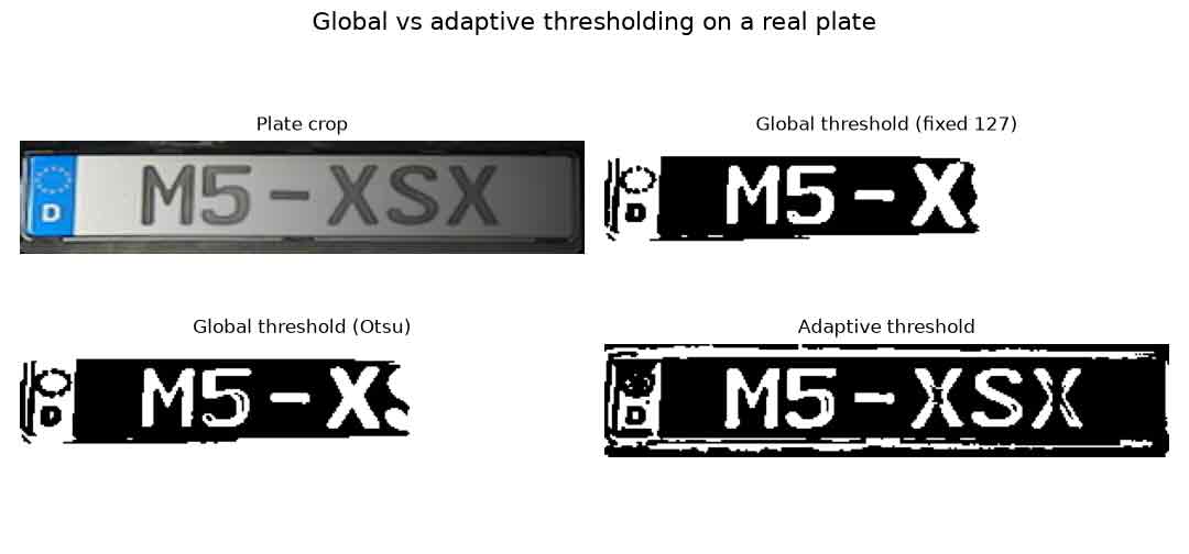
Figure 4. Why static thresholding fails. On a real plate with uneven lighting, the global threshold (fixed and Otsu) drops the characters on the shadowed side; adaptive thresholding keeps them all.

We use the inverted variant cv2.THRESH_BINARY_INV so that the characters come out white on a black background - the format cv2.findContours expects.

def adaptive_threshold(gray, block_size=config.ADAPTIVE_BLOCK_SIZE, c=config.ADAPTIVE_C):
    """Stage 2 - local thresholding robust to uneven lighting.

    Characters are darker than the plate, so THRESH_BINARY_INV produces white
    glyphs on a black background, which is what cv2.findContours expects.
    """
    if config.PRE_BLUR_KSIZE > 1:
        gray = cv2.GaussianBlur(gray, (config.PRE_BLUR_KSIZE, config.PRE_BLUR_KSIZE), 0)
    binary = cv2.adaptiveThreshold(
        gray, 255, cv2.ADAPTIVE_THRESH_GAUSSIAN_C, cv2.THRESH_BINARY_INV, block_size, c
    )
    # Light opening removes salt noise without eroding the strokes.
    kernel = np.ones((2, 2), np.uint8)
    binary = cv2.morphologyEx(binary, cv2.MORPH_OPEN, kernel, iterations=1)
    return binary

In line 1 the signature sets the parameters: block_size defaults to config.ADAPTIVE_BLOCK_SIZE (21, the 21 × 21 window) and c to config.ADAPTIVE_C (10), the constant subtracted from each local mean. Lines 2 to 6 are the docstring, noting why we invert the threshold. In line 7 and 8 an optional Gaussian blur (with kernel side config.PRE_BLUR_KSIZE = 3) suppresses pixel noise before thresholding. From line 9 to 11, cv2.adaptiveThreshold computes a separate threshold for every neighbourhood (cv2.ADAPTIVE_THRESH_GAUSSIAN_C) and, through cv2.THRESH_BINARY_INV, emits white glyphs on a black background. From line 12 to 14, a 2 × 2 morphological opening (cv2.MORPH_OPEN) removes isolated salt specks without thinning the strokes. Finally, line 15 returns the finished binary image.

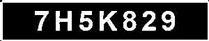
Figure 5. Stage 2 - white characters on a black background after adaptive thresholding.

6. Stages 3 & 4 - Contours and geometric filtering

Every white blob in the binary image is a contour candidate: the seven characters, but also noise specks, the plate border and the holes inside letters such as 8 and 0. We keep only the blobs whose geometry looks like a character, using simple rules on the bounding box:

• minimum / maximum width and height;
• minimum / maximum width-to-height ratio (aspect);
• a minimum area and a minimum fill ratio (fill = area ÷ bounding-box area);
• boxes that sit inside a larger accepted box (letter holes, the inner edge of the frame) are suppressed;
• finally, characters share a row and a roughly constant height, so boxes whose height or vertical centre disagree with the median - or that are separated from the rest by an abnormally large horizontal gap - are dropped as country bands, bolts or dirt.

Note that we call cv2.findContours with cv2.RETR_LIST (not cv2.RETR_EXTERNAL), so that characters sitting inside a plate frame are still returned; the frame itself is removed afterwards by its size.

def find_contours(binary):
    """Stage 3 - every white blob is a contour candidate.

    RETR_LIST (not RETR_EXTERNAL) so that characters sitting *inside* a plate
    frame are still returned; the frame itself is dropped later by its size.
    """
    contours, _ = cv2.findContours(binary, cv2.RETR_LIST, cv2.CHAIN_APPROX_SIMPLE)
    return contours


def _classify_box(contour):
    x, y, w, h = cv2.boundingRect(contour)
    area = cv2.contourArea(contour)
    aspect = w / h if h else 0.0
    fill = area / (w * h) if w * h else 0.0

    reason = ""
    if w < config.MIN_CHAR_WIDTH or w > config.MAX_CHAR_WIDTH:
        reason = "width"
    elif h < config.MIN_CHAR_HEIGHT or h > config.MAX_CHAR_HEIGHT:
        reason = "height"
    elif aspect < config.MIN_ASPECT or aspect > config.MAX_ASPECT:
        reason = "aspect"
    elif area < config.MIN_AREA:
        reason = "area"
    elif fill < config.MIN_FILL:
        reason = "fill"

    return CharBox(
        x=x, y=y, w=w, h=h, area=area, aspect=aspect, fill=fill,
        accepted=(reason == ""), reason=reason,
    )

From line 1 to 8, find_contours wraps cv2.findContours; the cv2.RETR_LIST flag in line 7 returns the blobs that sit inside the plate frame too, while cv2.CHAIN_APPROX_SIMPLE compresses each contour to its corner points. In line 12, cv2.boundingRect gives the box (x, y, w, h) of the blob. From line 13 to 15, the contour pixel area, the aspect ratio (w / h) and the fill ratio (area / (w * h)) are computed, where the if h else 0.0 guards avoid division by zero. From line 17 to 27, the geometric gate rejects the blob - and sets reason - when its width, height, aspect, area or fill fall outside the configured limits (config.MIN_CHAR_WIDTH = 3 … config.MIN_FILL = 0.10); an empty reason means it passed. Finally, from line 29 to 32, the result is packed into a CharBox where accepted is true only when no rule fired, and reason records which rule rejected it (used to colour Figure 6).

The higher-level filter_characters then sorts the accepted boxes by x and applies three more passes - _suppress_nested (drops letter holes and inner frames), _filter_by_consistency (drops height / row outliers) and _trim_isolated (drops boxes set apart by an abnormal gap) - which implement the last two bullet rules above.

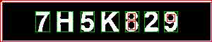
Figure 6. Stages 3-4 - green boxes are kept as characters; red boxes (the plate frame and the holes inside 8 and 9) are rejected by the geometric rules.

The accepted boxes are then sorted by their x coordinate, which is the natural reading order of the plate:

Figure 7. The seven isolated, clean characters that move on to feature extraction.

7. Stage 5 - Feature extraction in detail

A classifier cannot learn from raw pixels here; we describe each character with a compact, scale- and position-invariant feature vector of length 97. As planned, we start with two families of features - geometric and hue - and describe each one below.

Geometric features

• Hu moments (7 values) - seven nonlinear combinations of the normalised central moments that are invariant to translation, scale and rotation (the seventh also flips sign under reflection). Their raw values span many orders of magnitude, so we log-scale them with -sign(h)·log10|h| (the _hu_log helper). They summarise the overall mass distribution of the glyph - a coarse "shape fingerprint".
• Normalised central moments (7 values: nu20, nu11, nu02, nu30, nu21, nu12, nu03) - central moments divided by the area, which makes them translation- and scale-invariant. The second-order terms encode how wide or tall and how slanted the glyph is; the third-order terms encode its skew and asymmetry.
• Shape descriptors (3 values) - aspect (width / height) separates narrow glyphs like 1 from square ones like M; extent (ink area / bounding-box area) is high for filled glyphs and low for sparse ones; and solidity (ink area / convex-hull area) measures concavity, distinguishing open shapes like C and E from compact ones like O.
• Zoning densities (36 values) - the glyph is normalised to a 32 × 32 square and split into a 6 × 6 grid; each cell contributes the fraction of black pixels it contains. This is a coarse map of where the ink sits and is, in practice, the most discriminative block in the whole vector while staying robust to small noise.
• Projection profiles (32 values) - the horizontal projection (sum of ink per row) and the vertical projection (sum per column), each resampled to 16 bins and normalised. The horizontal profile reveals stacked bars - the three peaks of an E, for instance - while the vertical profile captures the left-to-right stroke layout.

Hue (colour) features

• The mean and standard deviation of the H, S and V channels over the character pixels, plus a small 6-bin hue histogram (12 values in total). These capture the plate's colour scheme (white, yellow, blue band, coloured text). On their own they barely identify a character, but they matter for a subtle reason: if the training glyphs were pure black-on-white their hue features would have almost zero variance, the StandardScaler would amplify that noise, and real coloured plates would then be mis-scaled. We therefore render the synthetic training glyphs on varied plate-like colours so the hue statistics carry realistic variance.

The geometric block is built by geometric_features:

def geometric_features(char_bin):
    """Geometric feature block computed from the binary character crop."""
    moments = cv2.moments(char_bin, binaryImage=True)

    h, w = char_bin.shape[:2]
    area = float(np.count_nonzero(char_bin))
    aspect = w / h if h else 0.0
    extent = area / (w * h) if w * h else 0.0

    cnts, _ = cv2.findContours(char_bin, cv2.RETR_EXTERNAL, cv2.CHAIN_APPROX_SIMPLE)
    if cnts:
        biggest = max(cnts, key=cv2.contourArea)
        hull_area = cv2.contourArea(cv2.convexHull(biggest))
        solidity = cv2.contourArea(biggest) / hull_area if hull_area else 0.0
    else:
        solidity = 0.0

    nu = np.array([
        moments["nu20"], moments["nu11"], moments["nu02"],
        moments["nu30"], moments["nu21"], moments["nu12"], moments["nu03"],
    ])

    norm_char = normalize_char(char_bin)
    return np.concatenate([
        _hu_log(moments),                 # 7
        nu,                               # 7
        [aspect, extent, solidity],       # 3
        _zoning_density(norm_char),       # ZONE_GRID**2
        _projection_profiles(norm_char),  # 2 * PROJECTION_BINS
    ])

In line 3, cv2.moments computes the image moments of the binary glyph; these feed both the Hu moments and the nu terms. From line 5 to 8 the basic shape descriptors are computed: aspect (w / h) and extent (ink area over bounding-box area). From line 10 to 16, the external contour's convex hull yields solidity (ink area / hull area), which captures concavity and falls back to 0 when no contour is found. From line 18 to 21, the seven normalised central moments nu20 … nu03 are collected. In line 23, normalize_char pads the glyph to a square and resizes it to config.CHAR_SIZE (32 × 32) so the zoning and projection features are scale-invariant. Finally, from line 24 to 30, the geometric blocks are concatenated: 7 log-Hu (_hu_log) + 7 nu + 3 shape + 36 zoning (_zoning_density, config.ZONE_GRID² = 6²) + 32 projection (_projection_profiles, 2 × config.PROJECTION_BINS = 2 × 16) = 85 values.

extract_features then appends the 12 hue values to give the final 97-D vector:

def extract_features(char_bin, char_color):
    """Full feature vector = geometric block + hue block."""
    return np.concatenate([
        geometric_features(char_bin),
        hue_features(char_color, char_bin),
    ]).astype(np.float32)

From line 3 to 6, the 97-dimensional vector is assembled as the 85-value geometric block (geometric_features) followed by the 12 hue values (hue_features: 6 HSV statistics plus a 6-bin hue histogram), cast to np.float32.

We deliberately begin with geometry and hue only; richer moment families such as Tchebichev and Zernike moments are easy to append to this same vector if accuracy ever proves insufficient.

8. Stage 6 - Learning and classification (SVM)

Training a classifier needs labelled character images. Rather than download and hand-label a dataset, we create the training set ourselves (in src/dataset.py): we render every character 0-9 and A-Z using about thirty installed system fonts, then augment each glyph with random rotation, shear, low-resolution blur, noise, stroke-width changes and plate-like colours. The label is free - it is the character we rendered, so no image is ever downloaded for training. Each synthetic glyph passes through the same binarise → crop → feature path used at inference time, so the training and test distributions match.

The features are standardised with StandardScaler and fed to a Support Vector Machine (RBF kernel) by default; a KNN and a small MLP neural network are selectable from the configuration.

def build_classifier(name=config.CLASSIFIER):
    """Scaler + classifier pipeline, selectable by name."""
    if name == "svm":
        clf = SVC(kernel="rbf", C=10.0, gamma="scale", probability=True)
    elif name == "knn":
        clf = KNeighborsClassifier(n_neighbors=3, weights="distance")
    elif name == "mlp":
        clf = MLPClassifier(hidden_layer_sizes=(128, 64), max_iter=600,
                            early_stopping=True, random_state=0)
    else:
        raise ValueError(f"Unknown classifier '{name}' (use svm|knn|mlp)")
    return Pipeline([("scaler", StandardScaler()), ("clf", clf)])

In line 1, name defaults to config.CLASSIFIER ("svm"). In line 4 the default model is created: an SVC with an RBF kernel, C = 10 and gamma = "scale", where probability=True enables per-character confidences. From line 5 to 9, the two alternatives selectable from config are built: a distance-weighted KNeighborsClassifier and a two-layer MLPClassifier. In line 11, an unknown name raises a ValueError. Finally, in line 12 the chosen classifier is wrapped behind a StandardScaler in a single Pipeline, so the 97 features are standardised before classification.

Training itself is one split followed by one fit:

X_tr, X_te, y_tr, y_te = train_test_split(
    X, y, test_size=0.2, random_state=0, stratify=y
)
pipeline = build_classifier(classifier)
pipeline.fit(X_tr, y_tr)

From line 1 to 3, train_test_split makes an 80/20 split of the synthetic samples; stratify=y keeps every class proportionally represented in both halves. In line 4 and 5 the pipeline is built and fit is called - the StandardScaler learns its mean and variance on X_tr, and the classifier then trains on the scaled features.

Results on synthetic data

Quantity	Value
Classes	36 (0-9, A-Z)
Synthetic training samples	~11,000
Feature dimension	97
Classifier	SVM (RBF)
Held-out validation accuracy	~99.4%

On clean cropped plates the full pipeline reads every character correctly:

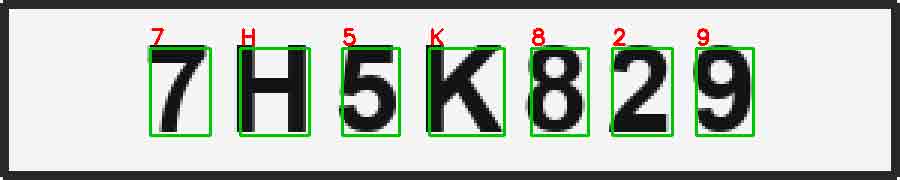
Figure 8. Stage 6 - each character classified and the plate read as 7H5K829.

9. Dataset

It helps to be precise about the two different image sets this project uses, because they are obtained in two different ways:

• Training images are created, not downloaded. The character classifier is trained entirely on the synthetic, font-rendered glyphs described in section 8 (src/dataset.py) - so no labelled character dataset is required and nothing is fetched from the network for training.
• Real sample / test scenes are downloaded. The real images in Figure 1 and the real plate crops used below are taken from the public OpenALPR Benchmark dataset (github.com/openalpr/benchmarks), which contains end-to-end European and US car photos with annotation files and is freely downloadable without registration. The helper script download_samples.py fetches each scene plus its .txt annotation, crops the plate region, and labels the crop with the ground-truth text. A larger annotated alternative is the Kaggle Car License Plate Detection dataset.

Both the downloader and the full source are in the project repository at github.com/babak-abad/Adhoc_OCR. These whole-scene datasets feed the detection step that crops the plate; the OCR in this article reads that crop.

Note that no images or trained model are committed to the repository - the data/ and models/ folders are git-ignored. After cloning you therefore build the data yourself, and it takes only two commands. First, python download_samples.py generates the synthetic test plates locally and (if you are online) downloads and crops the real OpenALPR scenes; run offline it simply skips the downloads, and the synthetic plates are enough to drive the whole pipeline. Second, python -m src.train renders the font-based training glyphs, caches them under data/cache/, fits the classifier, and saves models/ocr_model.joblib. Neither step needs a pre-existing labelled character dataset.

If you would rather use a different source, point SAMPLE_BASE_URL in your .env at any mirror of the OpenALPR benchmark layout, or download the Kaggle dataset above and drop the cropped plates into data/samples/ manually.

10. Running the project

# 0. clone the project
git clone https://github.com/babak-abad/Adhoc_OCR.git
cd Adhoc_OCR

# 1. install dependencies (inside a virtual environment)
pip install -r requirements.txt

# 2. download sample images + crop real plates + generate synthetic test plates
python download_samples.py

# 3. train the classifier (the learning stage)
python -m src.train --classifier svm

# 4. run the WHOLE project on one plate - no learning here
python run_pipeline.py --image data/samples/synthetic/plate_7H5K829.png

# 5. step-by-step stage images, and the real-world success/failure gallery
python steps/demo_steps.py --image data/samples/synthetic/plate_7H5K829.png
python steps/real_world.py

11. Real-world results: successes and failures

Synthetic accuracy is comforting but it is not the real test. We cropped the plate region of 24 real cars from the OpenALPR Benchmark (using the dataset's own bounding boxes), then ran the full pipeline on each. Figure 9 shows the outcome, ordered from best to worst, with the predicted text next to the ground truth.

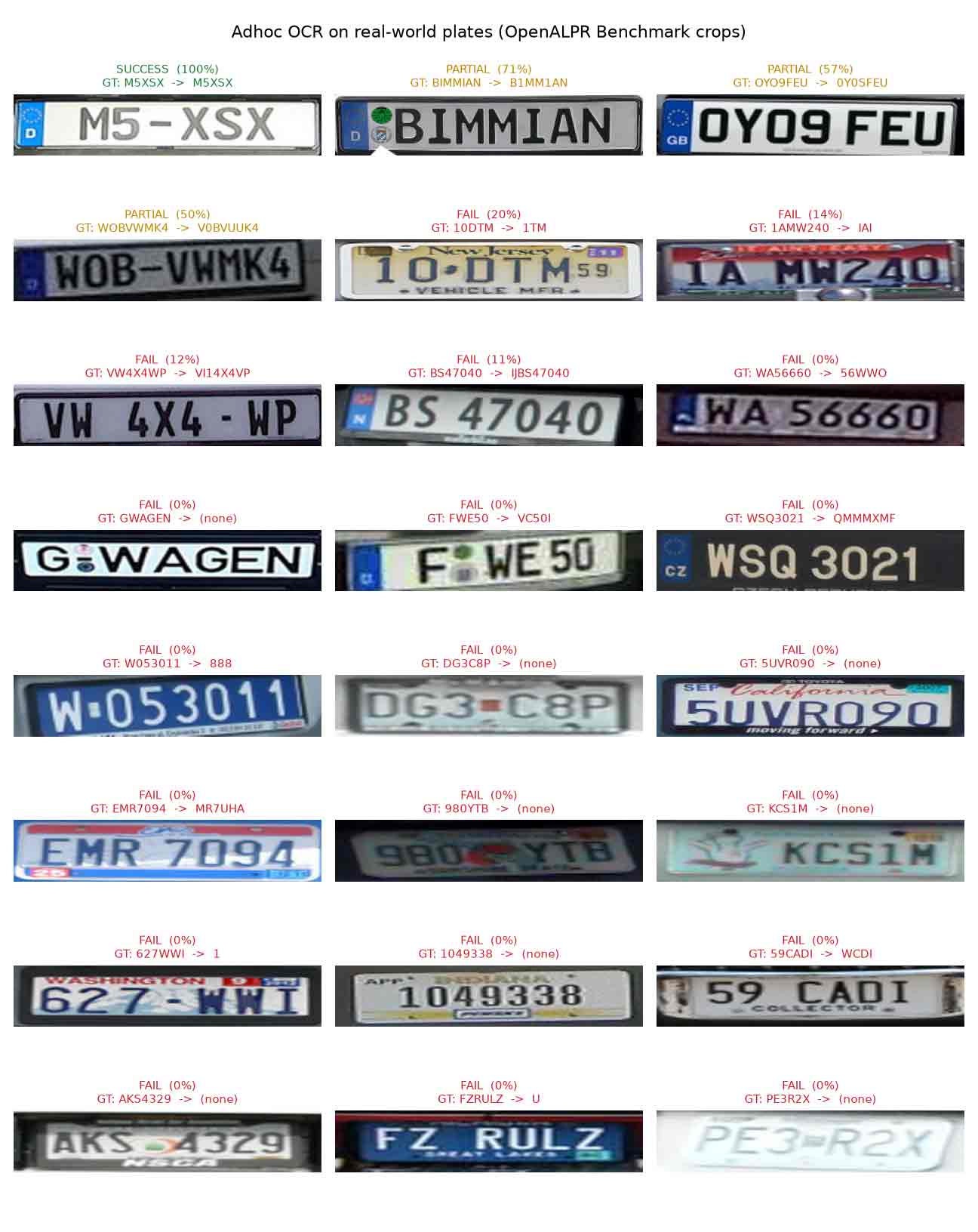
Figure 9. The adhoc model on real-world plates. Green = exact match, amber = most characters correct, red = failure.

The picture is honest and instructive:

• Successes - clean, high-contrast, well-cropped plates with an ordinary font are read perfectly, e.g. the German M5-XSX.
• Partial successes - many plates come out almost right: BIMMIAN, OYO9FEU and WOBVWMK4 each recover most of their characters, tripped up only by a single confusable pair such as I/1, O/0/D or W/V/U.
• Failures - low-resolution US plates, novelty / decorative fonts (FZ RULZ, KCS1M), faded / washed-out plates, and plates dominated by a coloured state banner either segment into noise or are misread entirely.

In other words, this adhoc strategy works on the easy third of real plates and struggles with the rest - which is exactly what we should expect from a hand-built classical pipeline and is the perfect motivation for the limitations below.

12. Limitations - what this adhoc model cannot handle

This model is intentionally simple and works best on clean, well-cropped, high-contrast Latin-script plates. It is not robust to the conditions a real-world ALPR system must survive. In particular it struggles or fails with:

• Blur - motion or out-of-focus blur merges strokes and breaks segmentation.
• Shadows and uneven lighting - adaptive thresholding helps (Figure 4) but strong shadows still defeat it.
• Dust, mud and dirt - occluding the glyphs adds spurious contours.
• Joined / connected characters - especially in cursive script languages (Persian, Arabic, Urdu), where letters connect, contour-based segmentation cannot split them.
• Washed-out or faded characters - low contrast makes thresholding drop parts of glyphs.
• Low resolution - small crops upscaled to 300 × 60 fragment into noise (several failures in Figure 9).
• Skew, rotation and perspective - a slanted plate breaks the left-to-right ordering and the size filters.
• Decorative / novelty fonts and non-Latin alphabets - the classifier is trained only on ordinary 0-9 and A-Z shapes.
• Touching the plate border, screws, flags and stickers - these add or merge contours.

Handling these robustly is exactly where modern deep-learning OCR (CNN + CTC or attention-based recognisers, trained on large real datasets) replaces the adhoc pipeline shown here. This project's value is clarity: every stage is visible and explainable, which makes it an excellent way to understand how classical OCR works before reaching for a heavier model.