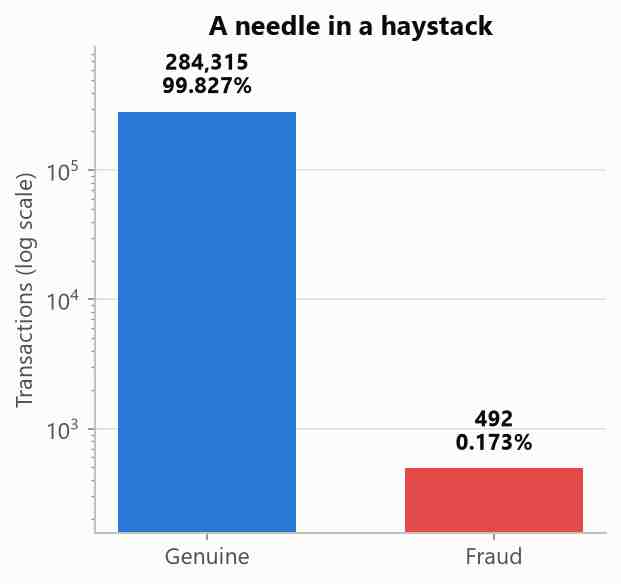
Fraud is a needle-in-a-haystack problem, and the haystack is enormous: in a public set of 284,807 real card transactions, exactly 492 are fraudulent — 0.173%, or one fraud for every 578 legitimate payments. At that ratio a model can score 99.8% accuracy by doing nothing at all, labelling every transaction “genuine,” so the metric everyone reaches for first is worse than useless here — it actively rewards the classifier that catches zero criminals. This article builds one that does catch them — an XGBoost model benchmarked honestly against logistic-regression and random-forest baselines — and walks through the code, the metrics, and the design choices that keep the extreme imbalance from quietly fooling us.
Code: github.com/babak-abad/Credit-Card-Fraud-Detection
The data: 284,807 transactions, 492 frauds
The dataset is the well-known ULB credit-card set[1], loaded here from OpenML (id 1597). Each row is one transaction described by 29 features: 28 components V1–V28 that have already been PCA-transformed to anonymise the original fields[2], plus the raw transaction Amount. The target column Class is 1 for fraud and 0 for genuine. The imbalance is so severe that a linear-scale bar chart cannot even render the fraud bar; Fig 1 puts both classes on a log scale so both are visible at once.
Loading and splitting the data
Two small functions read the file with pandas[3] and carve it into three partitions. Getting the split right matters more than usual: with 98 frauds riding on the outcome, a careless shuffle can leave a partition with almost none.
def load_data():
    frame = pd.read_csv(config.DATA_CSV)
    features = frame.drop(columns=[config.TARGET_COLUMN])
    labels = frame[config.TARGET_COLUMN].astype(int)
    return features, labels


def split_data(features, labels):
    x_train_full, x_test, y_train_full, y_test = train_test_split(
        features, labels,
        test_size=config.TEST_SIZE,
        stratify=labels,
        random_state=config.RANDOM_SEED,
    )
    x_train, x_val, y_train, y_val = train_test_split(
        x_train_full, y_train_full,
        test_size=config.VAL_SIZE,
        stratify=y_train_full,
        random_state=config.RANDOM_SEED,
    )
    return x_train, x_val, x_test, y_train, y_val, y_test
Lines 13–17 of src/data.py read the CSV and peel the Class column off as the label. Lines 20–33 then split twice using scikit-learn’s train_test_split[4]: line 21 holds out 20% as the untouched test set (56,962 rows, 98 frauds), and line 27 carves a further 20% off the remainder as a validation set (45,569 rows) used only for early stopping, leaving 182,276 rows to train on. The crucial arguments are stratify on lines 24 and 30, which preserves the exact 0.173% fraud rate in every partition, and the fixed random_state on lines 25 and 31, which makes the whole split reproducible.
A first signal: fraud hides in small amounts
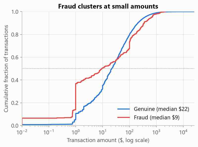
Before modelling, one exploratory cut already shows structure. Plotting the empirical CDF of transaction amounts for each class (log-x, so the small values spread out) reveals that fraud skews cheap: the median fraudulent charge is $9 versus $22 for genuine, and a large share of fraud sits at or below $1 — the classic “card tester” probing a stolen number with a tiny transaction before the big one, as Fig 2 makes visible.
Why accuracy is the wrong scoreboard
The test set contains 56,864 genuine transactions and 98 frauds. A do-nothing classifier that labels everything “genuine” gets 56,864 / 56,962 = 99.83% accuracy. Our XGBoost model gets 99.95%. Those two numbers are nearly identical, yet one model is worthless and the other catches three-quarters of all fraud. Accuracy simply cannot see the difference. Under heavy imbalance the honest metrics are the ones computed on the rare class:
- Precision — of the transactions we flag as fraud, how many really are? (The cost of false alarms.)
- Recall — of all real fraud, how much do we catch? (The cost of misses.)
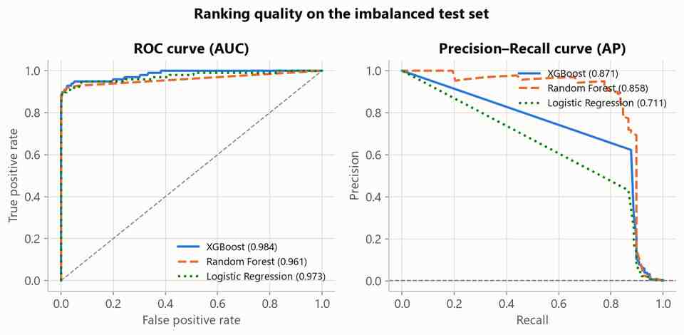
- PR-AUC (Average Precision) — the area under the precision–recall curve. Its random-chance baseline equals the fraud rate (0.0017), so a PR-AUC of 0.87 is roughly 500× better than chance — a claim ROC-AUC’s inflated 0.98 hides.
- MCC — a single balanced score that stays honest even when one class is 578× larger than the other.
A single evaluate function computes all of these for every model, keeping the threshold-dependent scores and the threshold-free ranking scores cleanly apart.
def evaluate(y_true, scores, threshold):
    """Threshold-independent and threshold-dependent scores for one model."""
    predictions = (scores >= threshold).astype(int)
    fpr, tpr, _ = roc_curve(y_true, scores)
    precision, recall, _ = precision_recall_curve(y_true, scores)
    thin_fpr, thin_tpr = thin_curve(fpr, tpr)
    thin_precision, thin_recall = thin_curve(precision, recall)
    matrix = confusion_matrix(y_true, predictions)
    return {
        "metrics": {
            "precision": float(precision_score(y_true, predictions)),
            "recall": float(recall_score(y_true, predictions)),
            "f1": float(f1_score(y_true, predictions)),
            "accuracy": float(accuracy_score(y_true, predictions)),
            "roc_auc": float(roc_auc_score(y_true, scores)),
            "pr_auc": float(average_precision_score(y_true, scores)),
            "mcc": float(matthews_corrcoef(y_true, predictions)),
        },
        "confusion_matrix": matrix.tolist(),
        "roc_curve": {"fpr": thin_fpr, "tpr": thin_tpr},
        "pr_curve": {"precision": thin_precision, "recall": thin_recall},
    }
Line 73 turns raw probability scores into hard 0/1 predictions at the decision threshold. The distinction that follows is the whole point: the threshold-dependent scores on lines 81–84 and 87 (precision, recall, f1, accuracy, mcc) read those hard predictions, whereas the ranking metrics on lines 85–86 (roc_auc and pr_auc) read the raw scores and ignore the threshold entirely. Lines 74–75 build the full ROC and precision–recall curves for later plotting; lines 76–77 hand them to thin_curve, a small NumPy[5] helper that down-samples each curve so the cached results file stays small. Every number the article reports comes out of this one function.
MCC (line 87) is worth pausing on, because it is the one score built from the whole confusion matrix at once. From true/false positives and negatives it is:
MCC = (TP × TN − FP × FN) / √((TP+FP)(TP+FN)(TN+FP)(TN+FN))
Because every one of the four cells appears in the numerator or the denominator, a model cannot win MCC by ignoring the rare class the way it can win accuracy — the huge true-negative count no longer drowns everything else out.
Three models, one honest comparison
XGBoost[6] is measured against two deliberately different baselines so the comparison is fair rather than flattering:
- Logistic Regression — a standardised linear model with class_weight="balanced". A transparent, fast reference point.
- Random Forest — 200 bagged trees, also class-balanced. A strong non-linear competitor that often matches boosting out of the box.
- XGBoost — gradient-boosted trees, tuned below.
def build_baselines():
    """The two reference models XGBoost is compared against."""
    log_reg = make_pipeline(
        StandardScaler(),
        LogisticRegression(
            max_iter=1000,
            class_weight="balanced",
            random_state=config.RANDOM_SEED,
        ),
    )
    random_forest = RandomForestClassifier(
        n_estimators=200,
        class_weight="balanced",
        n_jobs=-1,
        random_state=config.RANDOM_SEED,
    )
    return {"logistic_regression": log_reg, "random_forest": random_forest}
Lines 44–51 wrap logistic regression in a make_pipeline with a StandardScaler, because a linear model needs its inputs on a common scale; the tree models on lines 52–57 do not, so they take the raw features. Both baselines pass class_weight="balanced" (lines 48 and 54), which up-weights the rare fraud class in the loss — the standard scikit-learn answer to imbalance, and a useful contrast to the choice XGBoost makes below.
How gradient boosting works
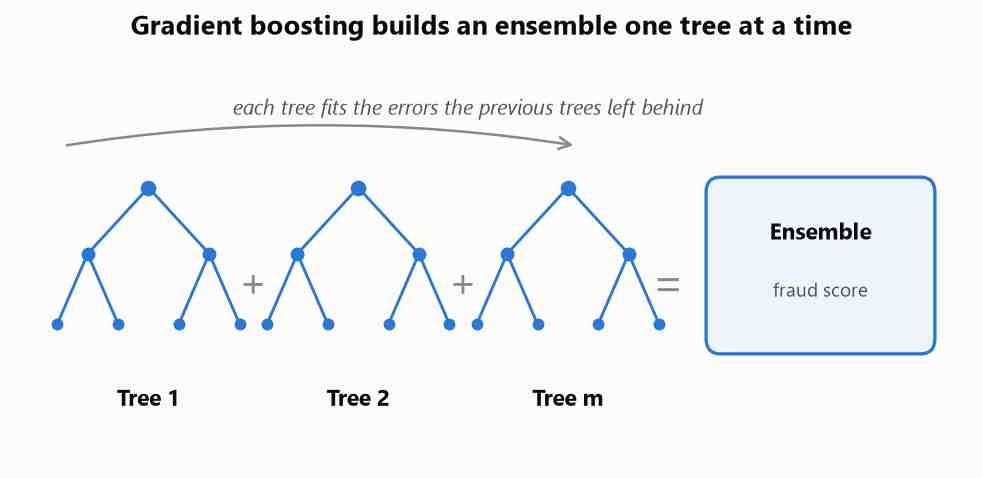
Where a random forest grows many independent trees and averages them, gradient boosting grows trees sequentially: each new tree is fit to the errors the ensemble has made so far, nudging the combined prediction a little closer each round, as sketched in Fig 3.
The whole configuration lives in one settings module, so a single edit changes the model everywhere it is built:
XGB_PARAMS = {
    "n_estimators": 400,
    "max_depth": 5,
    "learning_rate": 0.1,
    "subsample": 0.8,
    "colsample_bytree": 0.8,
    "min_child_weight": 1,
    "gamma": 0.0,
    "reg_lambda": 1.0,
    "objective": "binary:logistic",
    "eval_metric": "aucpr",
    "tree_method": "hist",
    "n_jobs": -1,
    "random_state": RANDOM_SEED,
}
EARLY_STOPPING_ROUNDS = 30
DECISION_THRESHOLD = 0.5       # probability cut-off for the positive (fraud) class

# Class-imbalance handling for XGBoost. The textbook recipe scale_pos_weight =
# n_genuine / n_fraud (~578 here) maximises recall but collapses precision and
# average precision. Selecting scale_pos_weight on validation AP prefers 1: the
# aucpr objective already ranks the rare class well, so no reweighting is used.
SCALE_POS_WEIGHT = 1.0
Line 29 sets a generous 400-tree ceiling that early stopping rarely reaches (see below), while lines 30–33 keep each tree shallow (max_depth 5) and each round conservative (a 0.1 learning_rate with 80% row and column sub-sampling) to hold overfitting in check. The single most important line is 38: "eval_metric": "aucpr" optimises the area under the PR curve, not accuracy, so the booster is graded on exactly the rare-class quality we care about. Lines 46–50 record a counter-intuitive decision. The textbook recipe for imbalance is scale_pos_weight = n_genuine / n_fraud (~578 here), which maximises recall but collapses precision and average precision, drowning analysts in false alarms. Because the aucpr objective already ranks the rare class well, selecting scale_pos_weight on validation Average Precision prefers 1.0 — no reweighting at all. Letting the loss function do the work beats brute-force reweighting.
Building the classifier is then a one-liner that splices those settings into the estimator:
def build_model(scale_pos_weight):
    return XGBClassifier(
        **config.XGB_PARAMS,
        scale_pos_weight=scale_pos_weight,
        early_stopping_rounds=config.EARLY_STOPPING_ROUNDS,
    )
Line 14 of src/model.py unpacks every hyper-parameter from config.py with **config.XGB_PARAMS, line 15 injects the chosen scale_pos_weight, and line 16 wires in early stopping. Nothing is hard-coded in the model file itself — every knob comes from the settings module.
Early stopping: letting the validation set choose the tree count
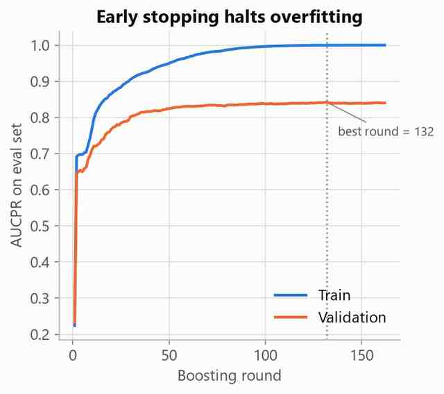
The 400-tree budget is an upper bound, not a target. After each boosting round the PR-AUC is measured on the validation set; when it fails to improve for 30 consecutive rounds (EARLY_STOPPING_ROUNDS), training halts and the best round is kept. Here it settled on iteration 131 — the 132nd tree — well short of the 400 cap, freezing the model where the validation curve peaks, as Fig 4 shows. The fit call is where the validation set enters:
    xgb = build_model(scale_pos_weight=scale_pos_weight)
    xgb.fit(
        x_train,
        y_train,
        eval_set=[(x_train, y_train), (x_val, y_val)],
        verbose=False,
    )
Line 144 passes an eval_set of two frames — the training split and the held-out validation split. XGBoost tracks aucpr on both after every round; the validation curve is the one early stopping watches, so the tree count is chosen by data the model never trained on rather than by a number picked in advance.
Results
With all three models fitted on the identical split, the headline comparison lines up in Fig 5. Every figure in this article is rendered from the cached results with Matplotlib[7].
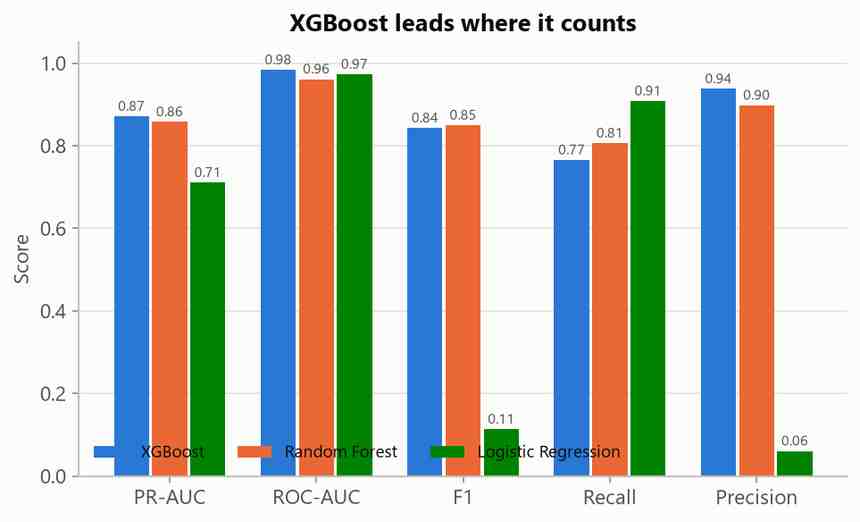
All numbers below are on the untouched test set, at the default 0.5 decision threshold. The best value in each row is bold.
| Metric | Logistic Regression | Random Forest | XGBoost |
|---|---|---|---|
| Precision | 0.060 | 0.898 | 0.938 |
| Recall | 0.908 | 0.806 | 0.765 |
| F1 | 0.113 | 0.849 | 0.843 |
| PR-AUC (Avg. Precision) | 0.711 | 0.858 | 0.871 |
| ROC-AUC | 0.973 | 0.961 | 0.984 |
| MCC | 0.231 | 0.851 | 0.847 |
| Accuracy | 0.976 | 0.9995 | 0.9995 |
The logistic-regression column is the cautionary tale. Its recall of 0.908 looks superb — it catches 89 of 98 frauds — but its precision is 0.060. To catch those 89 it raises 1,384 false alarms: roughly fifteen legitimate customers frozen for every real criminal caught. In production that is an unusable model, and no amount of headline “97.6% accuracy” rescues it.
Random Forest and XGBoost are genuinely close, and honesty demands saying so: the forest actually edges XGBoost on F1 (0.849 vs 0.843), MCC (0.851 vs 0.847) and recall. XGBoost wins where ranking quality matters most — PR-AUC (0.871) and ROC-AUC (0.984) — and on precision. Which model “wins” depends entirely on where you set the operating point, which is the next section’s subject.
ROC and PR curves: why the second one is the honest one
Plotting the two curve families side by side, in Fig 6, explains why the table can look so flattering. The ROC curves are all crowded into the top-left corner — under 578:1 imbalance almost any model looks excellent there, because the enormous true-negative count makes the false-positive rate tiny by construction. The precision–recall curve ignores true negatives entirely, so it is the one that separates the models and shows where precision falls off a cliff as you push for more recall. For rare-event detection, always read the PR curve.
The XGBoost confusion matrix
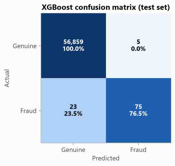
Fig 7 breaks the default-threshold decision down cell by cell. In raw counts, XGBoost catches 75 of the 98 frauds (recall 76.5%), misses 23, and raises only 5 false alarms out of 56,864 genuine transactions. That is the trade the default 0.5 threshold strikes: near-flawless precision at the cost of letting roughly a quarter of fraud slip through.
What the model keys on
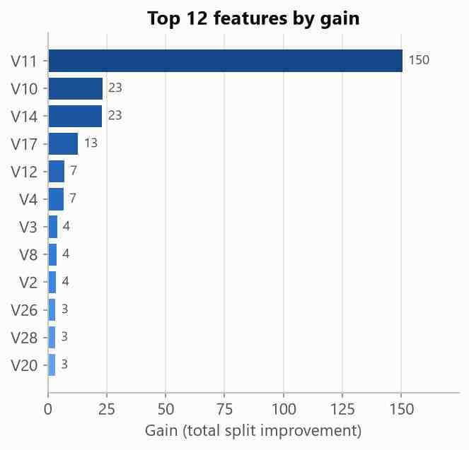
Importance by gain is heavily concentrated, as Fig 8 shows: V11 dominates, followed by V10, V14 and V17. Because the features are anonymised PCA components we cannot name what they represent, but the shape of the story is clear — fraud lives in a low-dimensional corner of the feature space, and the model finds it. (Gain-based importance is a property of the fitted model, not causal proof; SHAP values would be the next step for per-transaction explanations.)
The precision–recall dial
The single most important lever in a fraud system is not the algorithm — it is the decision threshold. Everything above used the default 0.5, which here favours precision. Lower the threshold and recall climbs (catch more fraud) while precision falls (more false alarms and blocked customers); raise it and the opposite happens. The right setting is a business decision, driven by the relative cost of a missed fraud versus a wrongly frozen card, not a statistical one. The value of a well-calibrated model like XGBoost is that its PR curve sits high enough to give you a genuinely useful range of operating points to choose from.
Key takeaways
- Never trust accuracy on imbalanced data. A 99.8%-accurate model here can be completely worthless. Judge on PR-AUC, MCC, and the precision/recall pair.
- Read the PR curve, not the ROC curve, for rare-event problems — ROC flatters everything.
- Let the objective handle imbalance before reaching for aggressive reweighting; here aucpr with scale_pos_weight = 1 beat the textbook 578× weight.
- Early stopping on a validation metric turned a 400-tree budget into a leaner, better-generalising 132-tree model for free.
- The threshold is the product. Model choice gets you a good PR curve; the operating point on it is where you actually trade misses against false alarms.
The complete, runnable code lives in the companion repository under src/, with every tunable — split ratios, hyper-parameters, the decision threshold — collected in config.py. Full attribution for the dataset and every library is in the repository’s RESOURCES.md.
Resources
Every dataset and library cited above — numbered in order of first appearance. The dataset is used under the license noted for its entry, and the derived figures in this article, rendered with Matplotlib, are derivative works of it. Click any bracketed marker such as [1] to jump to its entry.
- [1] Credit Card Fraud Detection dataset — Machine Learning Group, Université Libre de Bruxelles (ULB) & Worldline, Database Contents License (DbCL) 1.0. kaggle.com/datasets/mlg-ulb/creditcardfraud (also OpenML id 1597).
- [2] Dal Pozzolo, Caelen, Johnson & Bontempi, “Calibrating Probability with Undersampling for Unbalanced Classification” — IEEE Symposium Series on Computational Intelligence, 2015 (the dataset’s origin paper). ieeexplore.ieee.org/document/7376606
- [3] pandas — The pandas development team, BSD-3-Clause. pandas.pydata.org
- [4] scikit-learn — Pedregosa et al., JMLR 2011, BSD-3-Clause. scikit-learn.org
- [5] NumPy — Harris et al., Nature 2020, BSD-3-Clause. numpy.org
- [6] XGBoost — Chen & Guestrin, “XGBoost: A Scalable Tree Boosting System,” KDD 2016, Apache-2.0. github.com/dmlc/xgboost
- [7] Matplotlib — Hunter, Computing in Science & Engineering 2007, Matplotlib (BSD-compatible) license. matplotlib.org