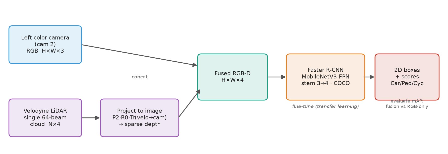
A camera gives a detector a crisp, coloured picture but no idea how far anything is; a LiDAR measures distance to the millimetre but paints only a sparse cloud of dots. Fuse the two and you get both — texture and geometry — which is why almost every self-driving stack carries both sensors. This article builds a working camera + LiDAR early-fusion 2D detector on KITTI[1], the classic autonomous-driving benchmark: it projects a single Velodyne scan onto a single colour camera, stacks the result into a 4-channel RGB-D image, and fine-tunes a pretrained detector on it. Then it measures exactly what the LiDAR channel buys you against a camera-only baseline.
Why KITTI, and why one camera + one LiDAR
There are richer fusion datasets, but for learning fusion KITTI is still the sweet spot. It is small, perfectly calibrated, ubiquitous in the literature, and it pairs a single 64-beam LiDAR with a forward colour camera — no radar, no six-camera rig to wrangle. Every requirement below maps straight onto it:
| Requirement | How KITTI meets it |
|---|---|
| Annotations | 2D and 3D boxes, plus per-frame calibration — everything fusion needs. |
| Easy / fast to train | ~7.5k labelled frames — a fine-tune, not a week-long job. |
| Strong community | The most-published fusion benchmark, so baselines and tutorials abound. |
| Transfer learning | Pretrained detectors drop straight in; we start from COCO weights. |
| Camera + LiDAR (not radar) | A 64-beam Velodyne and colour cameras — and no radar to complicate things. |
| Single camera + single LiDAR | One Velodyne and the left colour camera (cam 2) — the minimal fusion rig. |
One honest caveat up front: KITTI is a registered ~12 GB download, so to keep this tutorial reproducible on any machine the runnable figures below are rendered from a compact, self-contained synthetic scene written in the exact KITTI on-disk layout by src/make_demo_scene.py. The same src/ code — calibration, projection, dataset, training, evaluation — runs byte-for-byte on the real dataset the moment you point KITTI_ROOT at it. The whole pipeline is drawn in Fig 1.
Setup
python -m venv .venv
.venv\Scripts\activate                 # Windows
pip install -r requirements.txt        # torch, torchvision, numpy, matplotlib, pillow

# For an NVIDIA GPU, install the CUDA build of PyTorch instead:
pip install torch torchvision --index-url https://download.pytorch.org/whl/cu121

python src/make_demo_scene.py          # writes a KITTI-format demo to data/synthetic
Line 1 creates the virtual environment; line 2 activates it on Windows; line 3 installs the CPU dependencies; lines 5–6 are the one-line CUDA-build alternative for an NVIDIA GPU; line 8 writes the self-contained demo dataset. Skip line 8 and set KITTI_ROOT instead to train on the real thing.
The stack is PyTorch[2] and torchvision[3] for the detector and its COCO[4]-pretrained weights, with NumPy[5] doing the projection maths and Matplotlib[6] plus Pillow[7] rendering the figures. Every script runs from the project root and uses CUDA when it is available, falling back to the CPU otherwise.
Projecting one LiDAR onto one camera
Fusion starts with geometry. KITTI ships three pieces of calibration per frame: the camera projection matrix P2, the rectifying rotation R0_rect, and the rigid transform Tr_velo_to_cam that moves a point from the LiDAR frame into the camera frame. Chain them and a Velodyne point x lands at pixel P2 · R0_rect · Tr_velo_to_cam · x.
@dataclass
class Kitti_Calibration:
    p2: np.ndarray               # (3, 4) left colour camera
    r0_rect: np.ndarray          # (4, 4) rectifying rotation
    tr_velo_to_cam: np.ndarray   # (4, 4) velodyne -> camera

    @property
    def velo_to_image(self):
        return self.p2 @ self.r0_rect @ self.tr_velo_to_cam


def project_velo_to_image(points_velo, calib):
    xyz = points_velo[:, :3]
    ones = np.ones((len(xyz), 1), dtype=np.float32)
    projected = np.concatenate([xyz, ones], axis=1) @ calib.velo_to_image.T
    depth = projected[:, 2]
    front = depth > 1e-3
    uv = projected[front, :2] / depth[front, None]
    return uv, depth[front]
Lines 1–9 hold the calibration: three matrices, and a velo_to_image property (lines 8–9) that pre-multiplies them into one 3×4 matrix. Lines 12–19 do the projection: line 13 takes the point coordinates, lines 14–15 make them homogeneous and apply the matrix, line 16 reads off the camera-frame depth, line 17 keeps only points in front of the camera, and line 18 does the perspective divide to get pixel coordinates. The function returns both the pixels uv and their depth — and that depth is the signal the camera cannot supply.
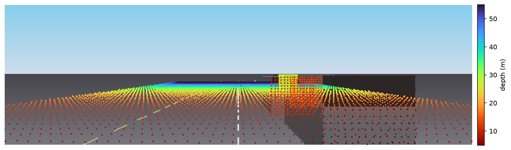
Painting that depth into an image-sized map gives the channel we will fuse. Empty pixels stay zero; where several points hit one pixel, the nearest wins so a car's surface is not erased by the ground behind it.
def build_sparse_depth_map(points_velo, calib, image_hw, max_depth_m=80.0):
    height, width = image_hw
    uv, depth = project_velo_to_image(points_velo, calib)
    u = np.round(uv[:, 0]).astype(int)
    v = np.round(uv[:, 1]).astype(int)
    inside = (u >= 0) & (u < width) & (v >= 0) & (v < height) & (depth < max_depth_m)
    u, v, depth = u[inside], v[inside], depth[inside]

    depth_map = np.zeros((height, width), dtype=np.float32)
    order = np.argsort(-depth)                 # far first, so nearer overwrites
    depth_map[v[order], u[order]] = depth[order]
    return np.clip(depth_map / max_depth_m, 0.0, 1.0)
Lines 4–5 round the projected pixels to integers; line 6 keeps only the ones inside the frame and closer than max_depth_m; line 9 starts an empty map; lines 10–11 write depths far-to-near so the closest return wins each pixel; and line 12 normalises to [0, 1]. The result is Fig 2: a sparse cloud of coloured depth landing exactly where the physical scene is.
Building the 4-channel fused input
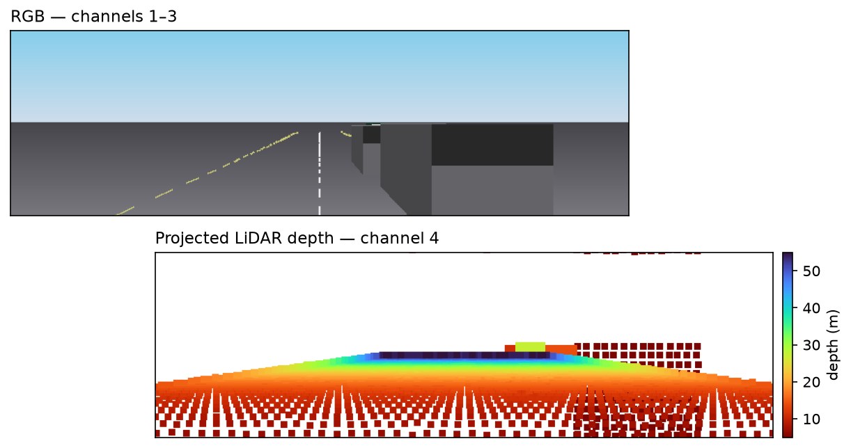
Early fusion is the simplest way to combine the two sensors: just stack the depth map onto the RGB image as a fourth channel and hand the detector a 4×H×W tensor. The dataset does exactly that per frame — and setting in_channels=3 gives the RGB-only baseline from the identical code.
rgb = np.asarray(Image.open(image_path).convert("RGB"), np.float32) / 255.0
channels = [torch.from_numpy(rgb.transpose(2, 0, 1))]        # (3, H, W)

if self.in_channels == 4:
    calib = parse_calib_file(calib_path)
    cloud = load_velodyne_bin(velodyne_path)
    depth = build_sparse_depth_map(cloud, calib, (height, width),
                                   max_depth_m=self.config.max_depth_m,
                                   dilation=self.config.depth_dilation)
    channels.append(torch.from_numpy(depth)[None])           # (1, H, W)

image = torch.cat(channels, dim=0)                           # (4, H, W)
Line 1 loads the image as a normalised float array; line 2 turns it into a 3-channel tensor. Lines 4–10 run only for the fusion model: they read the calibration and the cloud (lines 5–6), build the depth map (lines 7–9), and append it as a single extra channel (line 10). Line 12 concatenates everything into the 4-channel image. The two channel groups of that tensor are shown in Fig 3 — and note the low-contrast car in the RGB panel that nearly vanishes into the road yet stands out cleanly in depth.
Transfer learning: inflating the stem
We do not train from scratch. We start from a Faster R-CNN[8] with a MobileNetV3[9] backbone and an FPN[10] neck, already trained on COCO. There is one snag: a COCO model expects 3 input channels and we have 4. The fix is a standard trick — inflate the first convolution to accept the extra channel, copying the pretrained RGB filters and seeding the new depth filter with their mean so the network starts life behaving exactly like the RGB model.
def _inflate_stem(model, in_channels):
    old_conv = model.backbone.body["0"][0]            # first 3->16 conv
    new_conv = nn.Conv2d(in_channels, old_conv.out_channels,
                         kernel_size=old_conv.kernel_size, stride=old_conv.stride,
                         padding=old_conv.padding, bias=False)
    with torch.no_grad():
        new_conv.weight[:, :3] = old_conv.weight                        # keep RGB filters
        new_conv.weight[:, 3:] = old_conv.weight.mean(1, keepdim=True)  # seed the depth filter
    model.backbone.body["0"][0] = new_conv

in_features = model.roi_heads.box_predictor.cls_score.in_features
model.roi_heads.box_predictor = FastRCNNPredictor(in_features, num_classes)
Lines 2–5 build a fresh first convolution with in_channels inputs but the same shape otherwise; lines 7–8 are the heart of it — the first three input filters are copied verbatim from the pretrained weights, and the fourth is initialised to their channel mean, a neutral starting point for depth; line 9 swaps it into the backbone. Lines 11–12 replace the box predictor head so it outputs KITTI's classes (background + Car/Pedestrian/Cyclist) instead of COCO's 91. The detector's input normaliser is also widened to four channels so the depth channel is standardised alongside RGB. The RGB-only baseline runs this same builder with in_channels=3 and skips the inflation — so the two models differ by exactly one input channel.
Training
Because torchvision's detector returns its own loss dictionary in training mode, the loop is short: hand it images and targets, sum the losses it hands back, and step.
model = build_fusion_detector(num_classes=4, in_channels=in_channels).to(device)
params = [p for p in model.parameters() if p.requires_grad]
optimizer = torch.optim.SGD(params, lr=5e-3, momentum=0.9, weight_decay=5e-4)

model.train()
for epoch in range(1, num_epochs + 1):
    for images, targets in loader:
        images = [img.to(device) for img in images]
        targets = [{k: v.to(device) for k, v in t.items()} for t in targets]
        loss_dict = model(images, targets)         # rpn + box losses
        loss = sum(loss_dict.values())
        optimizer.zero_grad()
        loss.backward()
        optimizer.step()
Line 1 builds the fusion (or baseline) detector; lines 2–3 collect the trainable parameters and an SGD optimiser. Lines 6–7 loop over epochs and batches; lines 8–9 move the images and targets to the device; line 10 runs the model with targets, which puts it in training mode and returns the region-proposal and box losses; line 11 sums them; and lines 12–14 do the usual zero → backward → step. Training both models is two commands, then a third to score them:
python src/train.py                 # RGB-D fusion  -> checkpoints/fusion_detector.pt
python src/train.py --rgb-only      # RGB baseline  -> checkpoints/rgb_baseline.pt
python src/evaluate.py              # AP@0.5 and This email address is being protected from spambots. You need JavaScript enabled to view it. for both
Line 1 fine-tunes the 4-channel fusion model, line 2 the 3-channel baseline, and line 3 reports their Average Precision. On the demo scene (200 frames, a 160 / 40 train/val split) six epochs take a couple of minutes on a laptop GPU and the loss falls from about 0.78 to 0.53 for both.
Results: what the LiDAR channel buys
The two models are identical but for that one depth channel, so the gap between them is a clean measure of what fusion adds. Scored on the held-out validation frames:
| Model | AP@0.5 (Car) | |
|---|---|---|
| RGB-only baseline | 0.862 | 0.633 |
| RGB-D fusion | 0.904 | 0.773 |
Fusion wins at both thresholds, and the gap widens at the stricter
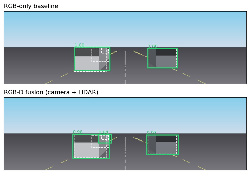
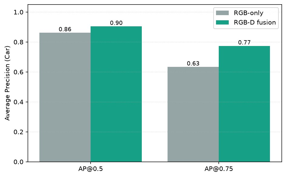
These are honest numbers from an easy synthetic benchmark, not a KITTI leaderboard entry — their job is to show the fusion mechanism paying off, end to end. On real KITTI the same code trains the same way; the absolute numbers change, the story does not. And this is only the gentlest form of fusion: stacking a depth channel is input-level fusion. Heavier schemes fuse LiDAR and camera features deeper in the network or lift everything into a shared bird's-eye-view space, and they win more — at the cost of the simplicity that makes this version trainable in minutes.
Key takeaways
- Fusion begins with calibration: chain KITTI's P2 · R0_rect · Tr_velo_to_cam to drop a single LiDAR scan onto a single camera image.
- Early fusion is just a channel stack: paint the projected depth into an image-sized map and concatenate it onto RGB to get a 4-channel input.
- Transfer learning survives the extra channel — inflate the first conv, copy the pretrained RGB filters, and seed the depth filter with their mean.
- The baseline is the same builder with in_channels=3, so the fusion-vs-RGB gap is a clean measurement of what LiDAR adds.
- Depth helps most with localisation and hard cases: the win grows at tighter IoU and it rescues low-contrast objects a camera-only model walks past.
The complete, runnable code — the calibration and projection in src/lidar_projection.py, the fused dataset in src/kitti_dataset.py, the stem-inflated detector in src/fusion_model.py, and src/train.py / src/evaluate.py / src/infer.py — lives in the companion repository. Run src/make_demo_scene.py to reproduce every figure without a download, or set KITTI_ROOT to train on the real dataset. Full attribution for every dataset and library is in the repository's RESOURCES.md.
Resources
Every dataset and library the implementation builds on — numbered in order of first appearance. The figures in this article are original renders of a synthetic scene generated in code, not KITTI imagery, so no dataset licence restricts their reuse here. Click any bracketed marker such as [1] in the text to jump to its entry.
- [1] KITTI — Geiger, Lenz & Urtasun, Are We Ready for Autonomous Driving? The KITTI Vision Benchmark Suite, CVPR 2012. Dataset released under CC BY-NC-SA 3.0 — non-commercial, research/education only; do not use KITTI or images derived from it on a commercial page. cvlibs.net/datasets/kitti
- [2] PyTorch — Paszke et al., An Imperative Style, High-Performance Deep Learning Library, NeurIPS 2019 (BSD-3-Clause style). pytorch.org
- [3] torchvision — models, weights & transforms (BSD-3-Clause). github.com/pytorch/vision
- [4] COCO — Lin et al., Microsoft COCO: Common Objects in Context, ECCV 2014. Source of the pretrained detector weights; annotations under CC BY 4.0, images per Flickr terms. cocodataset.org
- [5] NumPy — Harris et al., Array Programming with NumPy, Nature 2020 (BSD-3-Clause). numpy.org
- [6] Matplotlib — J. D. Hunter, Matplotlib: A 2D Graphics Environment, CiSE 2007 (Matplotlib license, BSD-style). matplotlib.org
- [7] Pillow (PIL fork) — image I/O (HPND / MIT-CMU license). python-pillow.org
- [8] Faster R-CNN — Ren et al., Towards Real-Time Object Detection with Region Proposal Networks, NeurIPS 2015. arXiv:1506.01497
- [9] MobileNetV3 — Howard et al., Searching for MobileNetV3, ICCV 2019. arXiv:1905.02244
- [10] FPN — Lin et al., Feature Pyramid Networks for Object Detection, CVPR 2017. arXiv:1612.03144