Texture is one of the oldest signals in remote sensing: long before deep networks, a forest could be told from a parking lot by the statistics of how neighbouring pixels vary. This article rebuilds that classical pipeline end to end — Haralick texture features read off the grey-level co-occurrence matrix — and puts a single 26-number texture fingerprint to work on real satellite scenes: retrieving look-alike tiles by distance, training a support-vector machine and a small neural net to name the scene, and letting two clustering algorithms find structure with no labels at all.
Code: Remote-sensing-Scene-Analysis-with-Haralick-Texture-Features
The dataset and a texture-only approach
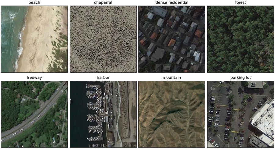
The NWPU-RESISC45 benchmark[1] holds 31,500 aerial scenes — 45 classes, 700 images each, every tile 256×256 pixels. To keep the demonstration fast and the figures legible, the project works with a curated subset of eight texturally-distinct classes — beach, chaparral, dense_residential, forest, freeway, harbor, mountain and parking_lot — sampled at 150 images per class for 1,200 tiles in total. The class list and every other tunable live in one config.py, so switching to all 45 classes is a one-line change. A sample of each class is shown in Fig 1.
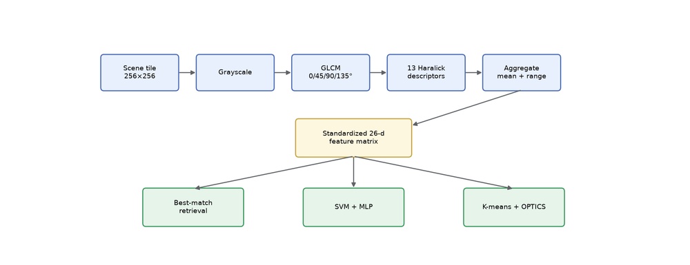
The whole approach here is deliberately classical: no convolutional network, no pretrained weights, no GPU. Each tile is reduced to a compact texture fingerprint, and everything downstream — retrieval, classification, clustering — operates on that fingerprint alone. The full route from a raw tile to the three tasks is sketched in Fig 2.
A note on licensing: NWPU-RESISC45 tiles are extracted from Google Earth and the dataset is distributed for research and educational use only. The scenes reproduced here are shown at reduced size for illustration; a commercial deployment would swap them for a commercially-licensed scene source.
Haralick features from the GLCM
The fingerprint starts with the GLCM. For a chosen offset — here one pixel — and a direction, it counts how often a pixel of grey level i sits next to a pixel of grey level j. Each such neighbour pair increments one cell of the matrix, so the GLCM is effectively a histogram of how tones are arranged beside one another. Fig 3 walks through the construction on a four-grey-level toy grid: counting every pair one pixel to the right populates the matrix, and the brightest cells mark the most frequent neighbouring-tone combinations.
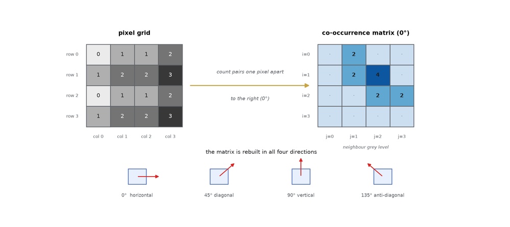
Texture is directional — the stripes on a ploughed field run one way, not all ways — so a single matrix would miss that structure. Instead the matrix is built at the four canonical directions: 0° (horizontal, neighbour to the east), 45° (diagonal), 90° (vertical, neighbour to the north) and 135° (anti-diagonal). These four angles span the principal axes along which texture repeats, and comparing the matrices across them is what lets the descriptors later tell a directional texture from an isotropic one. Fig 4 shows a freeway tile and its four co-occurrence matrices: the bright diagonal ridge means neighbouring pixels usually share a similar tone, and — because a road is strongly directional — its shape shifts noticeably between angles.
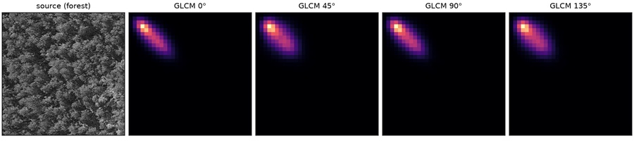
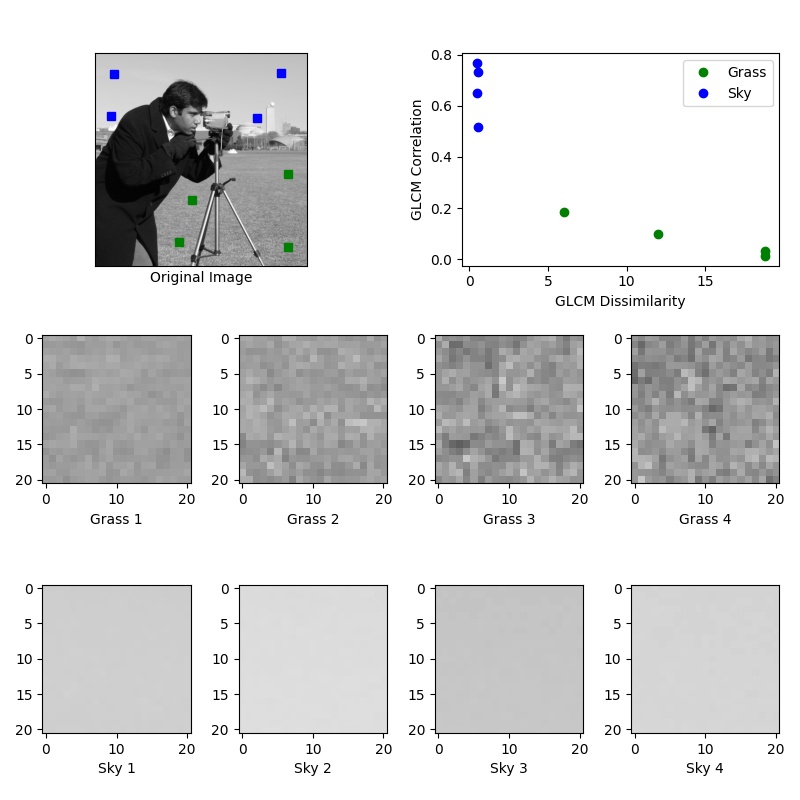
Another way to internalise the GLCM is to watch it respond to a known texture. Fig 5 pairs a roughly periodic surface with its co-occurrence matrix: bright, regularly spaced spots reveal that certain grey-level transitions repeat far more often than chance, while the diffuse background captures natural variability. This is the same histogram-of-neighbouring-tones idea of Fig 3, now on real pixel data rather than a toy grid.
contrast    = ∑i,j (i − j)2 p(i,j)
correlation = [ ∑i,j (i·j) p(i,j) − μiμj ] ÷ (σiσj)
Those two are representative, but the full set runs to thirteen. Each captures a different facet of how the co-occurrence probabilities are distributed — some measure overall uniformity, others the spread or disorder of tone differences, others again how strongly a neighbouring tone predicts the next. The complete list, in the order mahotas returns them, is:
| # | Descriptor | What it measures |
|---|---|---|
| 1 | Angular Second Moment | Uniformity — peaks when a few tone pairs dominate |
| 2 | Contrast | Local variation — how sharply neighbouring tones differ |
| 3 | Correlation | Linear dependence of neighbouring grey levels |
| 4 | Variance | Spread of the grey-level pair distribution |
| 5 | Inverse Difference Moment | Local homogeneity — high when nearby tones agree |
| 6 | Sum Average | Mean of the neighbouring-grey-level sums |
| 7 | Sum Variance | Spread of the sum distribution |
| 8 | Sum Entropy | Disorder in the sum distribution |
| 9 | Entropy | Overall randomness of the co-occurrence |
| 10 | Difference Variance | Spread of the neighbouring-tone difference distribution |
| 11 | Difference Entropy | Disorder in the difference distribution |
| 12 | Information Measure of Correlation 1 | Entropy-based correlation cue |
| 13 | Information Measure of Correlation 2 | Second entropy-based correlation cue |
The table above names each descriptor, but the formulas tell the fuller story. We adopt the standard notation of Haralick's paper: p(i,j) is the normalised co-occurrence probability at row i, column j; Ng is the number of grey levels; and the marginal sums Px(i) = ∑j p(i,j) and Py(j) = ∑i p(i,j) give the row and column distributions. Their means and standard deviations are μx, μy and σx, σy. Sums and differences are written Px+y(k) (probability that i+j = k) and Px−y(k) (probability that |i−j| = k). With this notation, the most widely used descriptors become:
| Descriptor | Formula | Intuition |
|---|---|---|
| Angular Second Moment | ∑i,j p(i,j)2 | Peaks when a few tone pairs dominate — a uniform, ordered texture |
| Contrast | ∑i,j (i−j)2 p(i,j) | Weights each pair by the squared grey-level gap; zero for a flat image |
| Correlation | [∑i,j (i·j) p(i,j) − μxμy] / (σxσy) | Linear predictability of a neighbour's tone; +1 for a perfect linear ramp |
| Inverse Diff. Moment | ∑i,j p(i,j) / [1+(i−j)2] | Local homogeneity; rewards neighbours that agree, gently penalises large gaps |
| Entropy | −∑i,j p(i,j) log p(i,j) | Overall disorder; maximal when every pair is equally likely |
| Sum Average | ∑k k · Px+y(k) | Mean of the neighbouring-grey-level sum distribution |
| Difference Entropy | −∑k Px−y(k) log Px−y(k) | Disorder of the neighbouring-tone difference distribution |
The thirteen descriptors are best understood in thematic groups. The first cluster — angular second moment and its close cousin entropy — measure how concentrated versus spread the co-occurrence distribution is. A smooth, repetitive texture packs probability into a handful of matrix cells, driving ASM high and entropy low; a rough, noisy texture flattens the distribution, inverting both. They are, in a sense, two views of the same information.
A second group — contrast and inverse difference moment — is sensitive to how sharply neighbouring tones differ. Contrast squares the gap (i−j)2 before weighting, so a few large jumps dominate the score; IDM does the opposite, dividing by 1+(i−j)2 so that agreeing neighbours contribute most. A parking lot's crisp edges push contrast up; a meadow's gentle gradients push IDM up.
Correlation stands apart: it asks whether a neighbour's grey level can be linearly predicted from the current pixel's. A ploughed field, where tone rises and falls along furrows, yields high correlation; an isotropic salt-marsh yields near zero. It is the one descriptor that captures directional linear structure rather than magnitude of variation.
The sum family — sum average, sum variance, sum entropy — describes the distribution of i + j, the total brightness of a neighbouring pair, while the matching difference family — difference variance, difference entropy — describes |i − j|, their local contrast. Together these marginal views let the fingerprint separate bright-uniform scenes (high sum average) from bright-rough ones (high difference entropy) even when the overall mean is similar.
Finally, the two information measures of correlation (IMC1, IMC2) are entropy-based alternatives to the linear correlation above: they compare the joint entropy of p(i,j) against the product of its marginals, capturing nonlinear dependencies that a Pearson-style correlation would miss. These are the descriptors most often dropped in lightweight implementations, but mahotas returns all thirteen, and keeping them costs nothing at inference time.
In code, the extraction lives in src/features.py. The mahotas[3] library builds the co-occurrence matrices at all four directions and returns the thirteen descriptors per direction in a single call.
def _per_angle_matrix(gray):
    """Return a (n_angles, n_descriptors) texture matrix for one grayscale image."""
    if config.feature_backend == "mahotas":
        import mahotas.features as mahotas_features

        return mahotas_features.haralick(gray, distance=config.glcm_distance)
Line 38 defines _per_angle_matrix; line 40 selects the backend; lines 41–43 build the co-occurrence matrices one pixel apart and return mahotas' Haralick matrix, shaped four directions by thirteen descriptors. A scikit-image[4] fallback (the rest of the function) computes a six-property GLCM subset when mahotas is unavailable, behind the same interface.
Four directions of thirteen descriptors is a 4×13 matrix per tile; to make one flat vector, the descriptors are averaged across the angles (a rotation-invariant summary) and concatenated with their per-angle range (which keeps the directional information). That yields the 26-number fingerprint.
def _aggregate(per_angle):
    """Collapse the per-angle matrix into one feature vector per config.feature_aggregation."""
    if config.feature_aggregation == "mean":
        return per_angle.mean(axis=0)
    if config.feature_aggregation == "all_angles":
        return per_angle.ravel()
    if config.feature_aggregation == "mean_ptp":
        return np.concatenate([per_angle.mean(axis=0), np.ptp(per_angle, axis=0)])
    raise ValueError(f"unknown feature_aggregation: {config.feature_aggregation!r}")
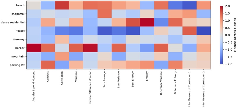
Line 59 opens _aggregate; lines 61–64 offer the mean-only and every-angle variants; lines 65–66 build the default 26-number vector by concatenating the per-angle mean with the per-angle range (np.ptp). Averaged over 1,200 tiles, these fingerprints already separate the classes by eye: Fig 6 shows harbor scoring high on angular second moment while forest sits low on entropy.
Extracting 1,200 fingerprints is the one slow step, so it is cached: the first run writes the feature matrix to disk, and every later run — retrieval, classification, clustering — reloads it instead of recomputing.
    if cache_path.exists() and not force:
        data = np.load(cache_path, allow_pickle=True)
        return data["X"], data["y"], data["paths"], feature_labels()

    paths, labels = dataset.list_samples()
    features = [
        extract_features(dataset.load_gray(path))
        for path in tqdm(paths, desc="Haralick features", unit="img")
    ]
Lines 110–112 short-circuit the whole run when a cache keyed to the current settings already exists; lines 114–118 otherwise list the sampled tiles and extract one fingerprint each. That cached matrix is the shared input to the three tasks that follow.
Finding the best-matched image
The simplest use of a fingerprint is retrieval: given one tile, find the scenes whose texture is closest. The 26 descriptors live on very different scales, so they are first z-scored; distance is then a plain Euclidean measure over the standardised vectors, computed in src/retrieval.py with SciPy's cdist.
def find_best_match(query_index, feature_matrix, metric=None, top_k=None):
    """Return the top-k nearest neighbours of one image in feature space.

    The query itself is excluded. Results are (index, distance) pairs sorted by
    increasing distance under the chosen metric.
    """
    metric = metric or config.retrieval_metric
    top_k = top_k or config.retrieval_top_k

    standardized = standardize(feature_matrix)
    query = standardized[query_index : query_index + 1]
    distances = cdist(query, standardized, metric=metric)[0]
    distances[query_index] = np.inf

    order = np.argsort(distances)[:top_k]
    return [(int(i), float(distances[i])) for i in order]
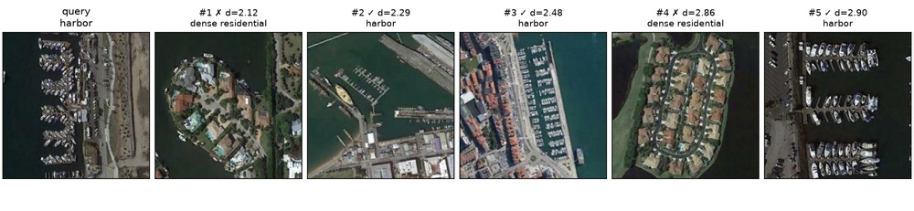
Line 15 defines find_best_match; line 24 z-scores the whole matrix; lines 25–26 measure the distance from the query row to every tile; line 27 pushes the query itself to infinity so it cannot match itself; lines 29–30 return the top_k nearest as (index, distance) pairs. Run for every tile, the neighbours share the query's label 68% of the time (precision@5). A worked example is in Fig 7: a harbor query pulls back three more harbors, and the two misses are dense-residential tiles whose grid of roofs is texturally close to a marina's grid of boats — an honest failure mode of a texture-only descriptor.
Classifying with an SVM and a simple ANN
With labels available, the fingerprints train a classifier. Two are compared in src/classify.py: a SVM with an RBF kernel, and a simple ANN — a two-layer MLP. Both are scikit-learn[5] estimators, each wrapped with a standardiser in one pipeline so scaling is learned on the training split alone.
    svm = make_pipeline(StandardScaler(), SVC(**config.svm_params))
    mlp = make_pipeline(
        StandardScaler(),
        MLPClassifier(random_state=config.random_seed, **config.mlp_params),
    )

    return {
        "class_order": class_order,
        "svm": _evaluate(svm, x_train, x_test, y_train, y_test, class_order),
        "mlp": _evaluate(mlp, x_train, x_test, y_train, y_test, class_order),
    }
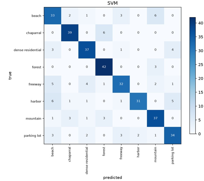
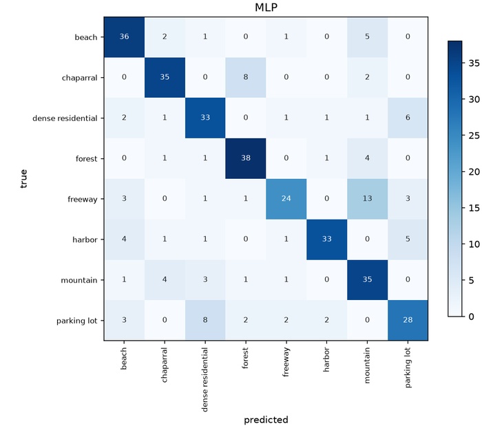
Line 40 wraps a StandardScaler and an RBF SVC in a single pipeline; lines 41–44 do the same for the MLPClassifier; lines 46–50 fit and score both on a held-out 30% test split and return their confusion matrices. On the eight-class subset the SVM edges ahead of the neural net:
| Model | Accuracy | Macro-F1 |
|---|---|---|
| SVM (RBF) | 0.79 | 0.79 |
| MLP (ANN) | 0.73 | 0.73 |
Where the errors fall is more telling than the headline number. The SVM confusion matrix in Fig 8 has a strong diagonal, with forest and chaparral almost never confused; the MLP in Fig 9 makes the same kinds of mistakes, spreading a little more mass off the diagonal. The recurring confusions — beach with mountain, harbor with parking lot — are exactly the pairs whose textures genuinely resemble one another.
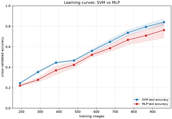
Before leaving the classifiers, it is worth asking how hungry each one is for data. Fig 10 traces both models' cross-validated accuracy as the training set grows from a fifth of the tiles to all of them. The SVM plateaus early — its RBF boundary is already well-placed within a few hundred examples — while the MLP climbs more slowly, the typical signature of a model with more weights to fit before it settles. Neither curve has fully flattened at 1,200 images, so both would likely keep gaining on the full 45-class dataset; on this eight-class subset the texture fingerprint is informative enough that the returns are already diminishing.
Clustering with K-means and OPTICS
Finally, the labels are set aside: can the fingerprints group the scenes on their own? Two contrasting methods run in src/cluster.py. K-means partitions every tile into a fixed number of clusters; OPTICS[6] instead follows local density, so it needs no cluster count and is free to label sparse tiles as noise.
    kmeans_labels = KMeans(
        n_clusters=config.kmeans_k,
        n_init=config.kmeans_n_init,
        random_state=config.random_seed,
    ).fit_predict(standardized)

    optics = OPTICS(
        min_samples=config.optics_min_samples,
        cluster_method=config.optics_cluster_method,
        eps=config.optics_eps,
    ).fit(standardized)
    optics_labels = optics.labels_
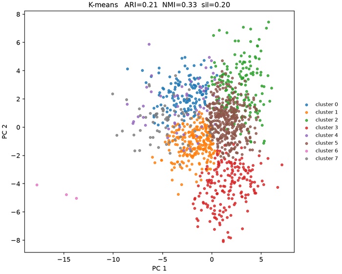
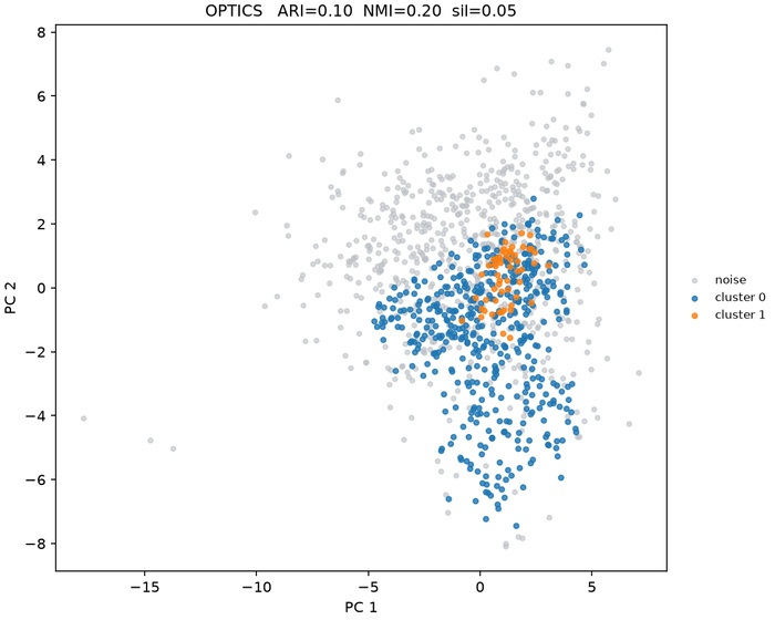
Lines 37–41 run K-means for the configured number of clusters; lines 43–47 run OPTICS, which takes no cluster count; line 48 reads back its labels, where density outliers come out marked −1. Scored against the true classes with the ARI and NMI, and internally with the silhouette, the two behave very differently:
| Method | Clusters | Noise | ARI | NMI | Silhouette |
|---|---|---|---|---|---|
| K-means | 8 | 0% | 0.21 | 0.33 | 0.20 |
| OPTICS | 2 | 57% | 0.10 | 0.20 | 0.05 |
Projected to two dimensions with PCA, K-means (Fig 11) carves the texture cloud into eight tidy partitions that line up loosely with the classes. OPTICS (Fig 12) tells the more honest story: the descriptors form one broad continuum rather than well- separated blobs, so it finds only two dense cores and consigns 57% of the tiles to noise. Texture alone orders these scenes but does not cleanly partition them.
Key takeaways
- A 26-number Haralick fingerprint, built from the GLCM at four angles, is enough to make real texture distinctions on satellite scenes — no deep network required.
- The same fingerprint serves three tasks unchanged: distance retrieval, supervised classification, and unsupervised clustering.
- Supervised, the texture baseline is respectable — roughly 0.79 accuracy for the SVM and 0.73 for the simple ANN on eight classes.
- Unsupervised, its limits show: K-means imposes tidy partitions, but density-based OPTICS reveals the descriptors form a continuum, not clean clusters.
- Texture-only features are a strong, interpretable classical baseline — the honest floor a learned representation has to beat.
The complete, runnable code for every figure and number above lives in the companion repository under src/, driven by a single config.py. Full attribution for the dataset and every library is in the repository's RESOURCES.md.
Resources
Every dataset, method and library cited above — numbered in order of first appearance. Sample scenes are used under the license noted for each; the derived images in this article are derivative works of them, except for the original GLCM schematic (Fig 3), which is the author's own diagram and carries no third-party copyright. Click any bracketed marker such as [1] to jump to its entry.
- [1] NWPU-RESISC45 — G. Cheng, J. Han, X. Lu, Proceedings of the IEEE, 2017; imagery from Google Earth, distributed for RESEARCH / EDUCATIONAL USE ONLY (not cleared for commercial republication). arxiv.org/abs/1703.00121
- [2] Haralick texture features — R. M. Haralick, K. Shanmugam, I. Dinstein, IEEE Trans. Systems, Man, and Cybernetics, 1973. doi.org/10.1109/TSMC.1973.4309314
- [3] Mahotas — L. P. Coelho, Journal of Open Research Software, 2013, MIT License. github.com/luispedro/mahotas
- [4] scikit-image — S. van der Walt et al., PeerJ, 2014, BSD-3-Clause. scikit-image.org
- [5] scikit-learn — F. Pedregosa et al., JMLR, 2011, BSD-3-Clause. scikit-learn.org
- [6] OPTICS — M. Ankerst, M. M. Breunig, H.-P. Kriegel, J. Sander, ACM SIGMOD, 1999. doi.org/10.1145/304182.304187
- [7] scikit-image GLCM gallery — S. van der Walt et al., scikit-image contributors, BSD-3-Clause licensed gallery example. The GLCM demo image (Fig 5) is a derivative work. scikit-image.org … plot_glcm