I trained five recurrent classifiers — a vanilla RNN, an LSTM, a GRU, a bidirectional LSTM, and a bidirectional LSTM with attention pooling — on a mixed corpus of 39,714 SMS messages and e-mails. Then I trained a TF-IDF vectorizer feeding a logistic regression, which fits in sixteen seconds on a CPU and beat all five.
Code: github.com/babak-abad/Spam-Detection
That result is the reason this article is worth reading. Along the way the models produce something better than a leaderboard: a measurement of exactly how far back in a message each architecture can actually see. The vanilla RNN, given a 200-token e-mail, turns out to depend on the last eight tokens and nothing else — not approximately, not mostly, but to four decimal places. The LSTM reaches back about thirty-four. The GRU reaches all the way to the first token. Every number in this article comes out of the repository; none of them are illustrative.
What a recurrent network is
A feed-forward network takes a fixed-size input. A message is not fixed-size. The recurrent answer[1] is to process the message one token at a time, carrying a hidden state vector ht forward from step to step, and to classify from the state left over at the end.
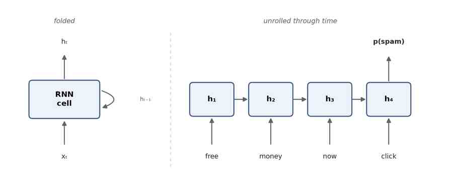
The unrolled picture in Fig 1 is the one to keep in your head, because it explains both why recurrent networks can handle variable-length input and why they are hard to train. Unrolled over 200 tokens, an RNN is a 200-layer network whose layers all share the same weights. Everything that goes wrong with very deep networks goes wrong here, and it goes wrong in a correlated way.
1. The corpus problem
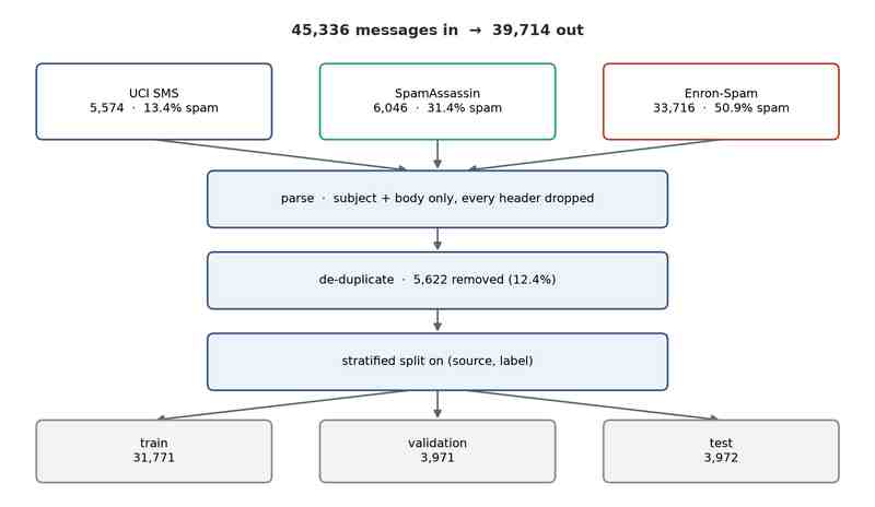
Most spam tutorials use one corpus. Using one corpus lets you avoid the only question that matters in practice, which is whether your filter survives contact with mail that does not look like your training set. So this project mixes three.
| Source | Messages | Spam rate | Kind |
|---|---|---|---|
| UCI SMS Spam Collection[2] | 5,574 | 13.4% | SMS |
| SpamAssassin public corpus[3] | 6,046 | 31.4% | e-mail (raw RFC 822) |
| Enron-Spam[4] | 33,716 | 50.9% |
These three disagree about nearly everything. SMS messages run a median of 12 tokens; SpamAssassin e-mails run 152; the longest Enron e-mail in the training split is 37,072 tokens. The spam rate ranges from 13% to 51%. A filter tuned on one of them is not a filter for the others, and the point of merging is to make that visible rather than to hide it.
What counts as “the message”
Only the subject line and the decoded body ever become text. Every header is dropped.
This is not fastidiousness, it is the difference between a real result and a fake one. The SpamAssassin corpus was machine-scored before it was published, so its X-Spam-Status and X-Spam-Level headers state the answer outright. Leave them in and your model learns to read the label off the input. Its routing headers are almost as bad: the spam and ham collections were gathered through different paths, so Received: chains alone separate the classes.
Body extraction prefers text/plain and falls back to text/html with tags stripped:
def extract_body(message):
    """Prefer text/plain, fall back to text/html stripped of tags."""
    plain, rich = "", ""
    for part in message.walk():
        if part.is_multipart():
            continue
        content_type = part.get_content_type()
        if content_type not in ("text/plain", "text/html"):
            continue
if content_type == "text/plain":
plain += payload + "\n"
else:
rich += payload + "\n"
return plain if plain.strip() else html_to_text(raw_html=rich)Line 83 walks every MIME part while lines 84–85 skip the multipart containers, which carry no text of their own. Lines 86–88 discard anything that is not one of the two body types. Lines 89–97, omitted between the two blocks, decode the payload — they exist only to survive the corpus’s broken charset declarations. Lines 98–101 accumulate the two kinds of body separately, and line 102 states the preference: the plain text when there is any, otherwise the HTML with its tags stripped.
De-duplicate before you split
The Enron mirror carries duplicate e-mails — forwards, replies quoting the whole thread, mailing list copies. If a message lands in the training split and its twin lands in test, the test score measures memorization and reports it as accuracy.
So de-duplication happens first, on the merged frame, before anything is split. Two passes: an exact hash of the whitespace-collapsed lowercase text, then a “near” hash that additionally strips punctuation and digits.
def near_key(text):
    stripped = PUNCT_DIGIT_RE.sub(" ", text.lower())
    collapsed = WHITESPACE_RE.sub(" ", stripped).strip()
    return hashlib.sha1(collapsed.encode("utf-8")).hexdigest()
Line 149 replaces every character that is not a lowercase letter or whitespace — punctuation and digits both — with a space, so a forward that differs only in a quoted timestamp collapses onto its original. Line 150 squeezes the resulting runs of whitespace down to one. Line 151 hashes what is left, which is what the de-duplicator groups on.
That removes 5,622 messages, 12.4% of the corpus. The splits are then stratified on the (source, label) pair rather than on the label alone, so each split preserves both the class balance and the source mix, and a final assertion checks that no content hash appears in two splits.
The result: train 31,771 · validation 3,971 · test 3,972, each 41.9% spam. Note what that number implies — a model that predicts “ham” for everything scores 58.1% accuracy. Keep it in mind when you see 94%.
Length
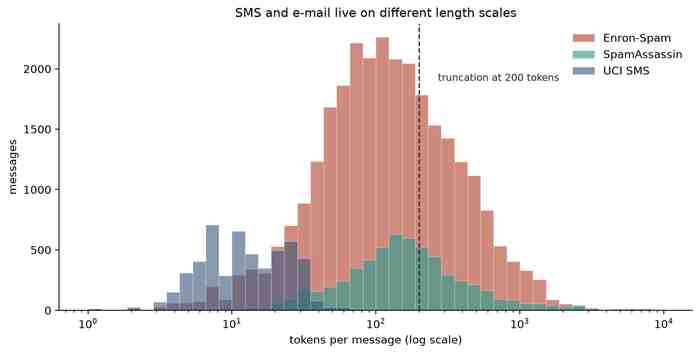
Sequence length has to be capped somewhere, and this project caps it at 200 tokens. Fig 2 shows why that single number lands so unevenly, and the table puts figures on it:
| Source | Median tokens | Mean | Longest | Truncated at 200 |
|---|---|---|---|---|
| UCI SMS | 12 | 15.5 | 189 | 0.0% |
| SpamAssassin | 152 | 302.7 | 14,628 | 36.8% |
| Enron-Spam | 117 | 243.2 | 37,072 | 31.6% |
Over the whole training split, 28.3% of messages get truncated. And truncation keeps the first 200 tokens (ids[:max_len]), discarding the tail. Remember this; it comes back with a vengeance in section 3, and again in section 10 where it turns out to have quietly handicapped every neural model against the baseline.
2. From text to tensors
Masking
Spam signals through the presence of a link, a phone number, or a currency amount far more than through the literal string. http://bit.ly/x2f and http://tinyurl.com/9dk2 are the same feature. Keeping them distinct wastes vocabulary on tokens that will each be seen once.
So five regexes collapse them to placeholders, in an order that matters — URLs before e-mails, because a URL can contain @; both before bare numbers.
# Order matters: URLs before e-mails (a URL can contain '@'), both before numbers.
URL_RE = re.compile(r"https?://\S+|www\.\S+")
EMAIL_RE = re.compile(r"\S+@\S+\.\S+")
PHONE_RE = re.compile(r"\+?\d[\d\-\s()]{7,}\d")
CURRENCY_RE = re.compile(r"[$£€]\s?\d[\d.,]*")
NUMBER_RE = re.compile(r"\b\d+([.,]\d+)*\b")
TOKEN_RE = re.compile(r"[a-z<][a-z0-9<>_']*")
Line 12 records the constraint that the ordering encodes, because nothing else in the code enforces it. Lines 13–17 are applied in exactly that order, each collapsing its match to a single placeholder. Line 18 is the tokenizer, and its character class is the part worth pausing on: it admits < and >, which is what keeps a placeholder such as <url> intact as one token instead of shattering into three.
Run it on a message:
raw     WINNER!! Claim your £1000 prize now at http://bit.ly/x2f
masked  winner!! claim your <cur> prize now at <url>
tokens  ['winner', 'claim', 'your', '<cur>', 'prize', 'now', 'at', '<url>']
ids     [2399, 673, 18, 27, 970, 79, 30, 51]
Line 1 is the raw message. Line 2 shows the currency amount and the URL replaced by placeholders and the whole string lowercased. Line 3 is what the tokenizer keeps — note that the trailing punctuation of “winner!!” is gone while the placeholders survive whole. Line 4 is the integer sequence the embedding table actually receives.
Masking is also what lets a single vocabulary span SMS and e-mail at all. “Txt 85233 to claim GBP1000” and “click http://…” become structurally similar once the payload is <num>, <cur> and <url>.
It works almost too well. <num> is, by a wide margin, the most common token in the training corpus:
| Token | Train count | ID |
|---|---|---|
| <num> | 339,172 | 2 |
| the | 257,180 | 3 |
| to | 186,996 | 4 |
| <cur> | 32,175 | 27 |
| <phone> | 16,877 | 40 |
| <url> | 13,515 | 51 |
| <email> | 5,681 | 133 |
There are more <num> tokens than there are instances of the word “the”. A quirk of the regex is partly responsible: 12:30 contains no colon in NUMBER_RE’s pattern, so it masks to two separate <num> tokens rather than one time-of-day token. That is a small design smell, and section 7 shows the attention model tripping over it.
The vocabulary
Built from the training split only — counting tokens across validation or test leaks their vocabulary into the model, which is a subtle enough leak that it is worth being explicit about.
@classmethod
def build(cls, texts, min_freq=config.MIN_FREQ, max_size=config.MAX_VOCAB):
    counter = Counter()
    for text in texts:
        counter.update(tokenize(text=text))

    stoi = {config.PAD_TOKEN: config.PAD_IDX, config.UNK_TOKEN: config.UNK_IDX}
    eligible = [(token, count) for token, count in counter.most_common() if count >= min_freq]
    for token, _ in eligible[: max_size - len(stoi)]:
        stoi[token] = len(stoi)
    return cls(stoi=stoi)
Lines 27–29 count every token in the training texts and nowhere else. Line 31 seeds the mapping with the two reserved tokens so that padding keeps index 0 and the unknown token index 1. Line 32 keeps only tokens seen at least min_freq times, ordered by frequency, and line 33 truncates that list to the vocabulary budget. Line 35 hands back the finished mapping.
With a floor of min_freq=2 and a cap of 20,000, the cap binds: the vocabulary is exactly 20,000 tokens. Everything else maps to <unk>. On the test split that is 5.97% of tokens, with a median per-message rate of 3.00% — high enough to matter, and a direct consequence of merging corpora whose vocabularies barely overlap.
Padding, packing, truncation
Batches pad to the longest message in the batch, not to the global 200:
def pad_collate(batch):
    sequences, lengths, labels = zip(*batch)
    max_len = max(lengths)
    padded = torch.full((len(sequences), max_len), config.PAD_IDX, dtype=torch.long)
    for row, sequence in enumerate(sequences):
        padded[row, : len(sequence)] = sequence
    return (
        padded,
        torch.tensor(lengths, dtype=torch.long),
        torch.tensor(labels, dtype=torch.float),
    )
Line 32 takes the longest length present in this batch, not the global cap. Line 33 allocates a block filled entirely with the pad index, and lines 34–35 overwrite the leading positions of each row with the real tokens, leaving the tail as padding. Lines 36–40 return the padded block alongside the true lengths, and those lengths are what the model needs in order to ignore everything it just padded.
A batch of SMS messages then costs about 20 time steps instead of 200. The padded positions still have to be kept out of the recurrence, which is what pack_padded_sequence does — every model in this project runs its core on a packed sequence, so the final hidden state is the state after the last real token, not after fifty pad tokens.
def _pack(embedded, lengths):
    return pack_padded_sequence(embedded, lengths.cpu(), batch_first=True, enforce_sorted=False)
Line 20 is the whole mechanism: the lengths move to the CPU because the packing bookkeeping happens there, and enforce_sorted=False lets the batch arrive in any order rather than pre-sorted by length.
Get this wrong and short messages in a long batch get classified from their padding. It is the most common silent bug in recurrent text models.
3. The recurrent core, and where it breaks
The vanilla RNN
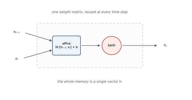
ht = tanh( Wih xt + Whh ht−1 + b )
In PyTorch[5] the entire model is a dozen lines:
class Simple_RNN(_Recurrent_Base):
    """Vanilla tanh RNN. Needs gradient clipping: on 200-token e-mails the
    unrolled gradient explodes as readily as it vanishes."""

    def __init__(self, vocab_size):
        super().__init__(vocab_size=vocab_size, head_in=config.HIDDEN_DIM)
        self.core = nn.RNN(
            config.EMBED_DIM, config.HIDDEN_DIM,
            num_layers=config.NUM_LAYERS, batch_first=True, nonlinearity="tanh",
        )

    def forward(self, x, lengths):
        _, hidden = self.core(_pack(embedded=self.embedding(x), lengths=lengths))
        return self.classify(features=hidden[-1])
Lines 42–45 are the recurrent core and nothing more; the embedding, the dropout and the linear head all live in the shared base class. Line 48 packs the embedded batch and runs it, discarding the per-step outputs and keeping only the final hidden state. Line 49 classifies from hidden[-1], the state after the final token. So every token’s contribution must survive, in that one 128-dimensional vector, all the way to the end of the message.
Consider what backpropagation asks of this. The gradient of the loss with respect to an early hidden state ht has to travel back through every step between t and the end:
∂hT / ∂ht = ∏k=t+1T diag( tanh′(ak) ) Whh⊤
It is a product of T − t matrices. Since tanh′(·) ≤ 1 everywhere and is strictly less than 1 away from the origin, each factor shrinks the gradient a little. Over 200 steps, “a little” 200 times compounds into annihilation. This is Hochreiter’s 1991 vanishing gradient[6], and Bengio, Simard and Frasconi’s 1994 analysis of it[7].
That is the textbook argument. It is also usually where the textbook stops. Let’s measure it.
Measuring the vanishing gradient
Take the 64 test messages long enough to fill the entire 200-token window. Push each through the trained checkpoint, backpropagate the output logit, and record the norm of the gradient arriving at the embedding of each position t. That norm is exactly “how much does the model’s decision depend on the token at position t”, as the optimizer sees it. Median gradient norm by position:
| Model | t=1 | t=25 | t=50 | t=100 | t=150 | t=190 | t=200 |
|---|---|---|---|---|---|---|---|
| Simple RNN | 0.0 | 0.0 | 0.0 | 0.0 | 2.9e-13 | 2.7e-03 | 8.6e-01 |
| LSTM | 8.5e-05 | 1.3e-04 | 2.1e-04 | 5.1e-04 | 6.4e-03 | 7.4e-02 | 1.2e+00 |
| GRU | 6.1e-02 | 1.0e-02 | 1.1e-02 | 9.9e-03 | 1.6e-02 | 5.7e-02 | 8.9e-01 |
Those zeros are not rounding. In the vanilla RNN the gradient reaching position 1 is exactly 0.0 in float32, in all 64 of 64 messages. Somewhere between position 100 and position 150 the product underflows past the smallest representable float and stays there. If you ask how many positions carry at least 1% of the peak gradient, the answer for the vanilla RNN is a median of 8 positions out of 200, the earliest of them at position 193.
The LSTM’s gradient decays too — by a factor of 14,319 from the last token to the first — but it never reaches zero. About 34 positions clear the 1% bar, the earliest at 156.
The GRU barely decays at all. From position 200 back to position 1 the gradient falls by a factor of 15, and 138 of 200 positions clear the 1% bar, reaching all the way back to the first token.
An occlusion check
Gradients tell you about the local slope of the decision function, which is not quite the same as what the model actually uses. So here is an independent test that does not involve derivatives at all: replace a span of the message with <unk> and see how far the output logit moves. (The logit, not the probability — these models are so confident that the sigmoid saturates and hides everything.) Median absolute logit shift over the same 64 messages, as a fraction of the model’s median absolute logit:
| Model | blank the first 100 tokens | blank the last 8 tokens |
|---|---|---|
| Simple RNN | 0.00% | 60.24% |
| LSTM | 1.32% | 29.80% |
| GRU | 10.56% | 38.48% |
Deleting half the message — the first hundred tokens — moves the vanilla RNN’s logit by 0.0000. Not “slightly”. It does not move. Deleting the last eight tokens moves it by 60% of its magnitude.
Two independent measurements — one of the backward pass, one of the forward pass — put the three models in the same order and agree on how stark the gap is. The vanilla RNN classifies long e-mails by reading eight tokens.
And now recall that truncation keeps the first 200 tokens of a message. So for a long e-mail, the vanilla RNN’s decision rests on tokens 193 through 200 — an essentially arbitrary eight-word window somewhere in the opening paragraph, chosen by nothing but where the truncation happened to land.
The genuinely surprising thing is that this still gets 94% accuracy. Spam is so redundantly marked that almost any window of it will do. That fact will matter in section 10.
4. The LSTM: a path that isn’t a product
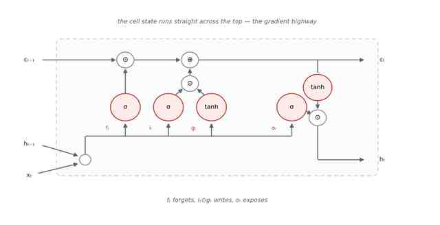
Hochreiter and Schmidhuber’s 1997 answer[8] was to add a second state vector, the cell state ct, and to give it a path through time that is additive rather than multiplicative:
ft = σ( Wf [ht−1, xt] + bf )        forget
it = σ( Wi [ht−1, xt] + bi )        input
gt = tanh( Wg [ht−1, xt] + bg )     candidate
ot = σ( Wo [ht−1, xt] + bo )        output

ct = ft ⊙ ct−1 + it ⊙ gt              cell state
ht = ot ⊙ tanh( ct )                  hidden state
The whole trick is the fifth line. ∂ct / ∂ct−1 = ft, a number the network chooses, per dimension, per step. If it wants to remember something for 200 steps it sets ft near 1 in that dimension and the gradient passes through unattenuated. Nothing forces the product to shrink. The forget gate — which Hochreiter and Schmidhuber did not have; Gers, Schmidhuber and Cummins added it in 2000[9] — is what lets the cell also discard, so the state does not saturate.
Three gates reading the same concatenated [ht−1, xt], plus a candidate, is four times the recurrent weights of a vanilla RNN: 132,096 parameters against 33,024.
5. The GRU: the same idea, cheaper
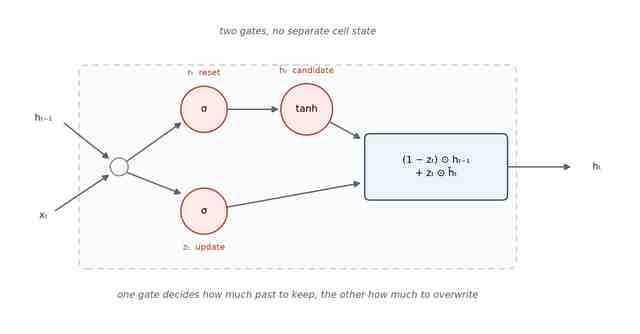
Cho et al. (2014)[10] asked whether all of that machinery is necessary and concluded it mostly is not. The GRU drops the separate cell state and merges the forget and input gates into a single update gate:
rt = σ( Wr [ht−1, xt] + br )                 reset
zt = σ( Wz [ht−1, xt] + bz )                 update

h̃t = tanh( Wh [rt ⊙ ht−1, xt] + bh )      candidate
ht = (1 − zt) ⊙ ht−1 + zt ⊙ h̃t          new state
The last line is a convex interpolation. Setting zt ≈ 0 copies the previous state forward untouched — an identity path, the same gradient highway the LSTM builds with ft, expressed in one gate instead of two. Three gate-sized weight blocks instead of four: 99,072 recurrent parameters.
A footnote for anyone reading the PyTorch source: nn.GRU implements ht = (1 − zt) ⊙ nt + zt ⊙ ht−1, with zt multiplying the old state rather than the candidate. It is the same function with z replaced by 1 − z, and the learned weights simply absorb the flip. The equations above follow Cho et al.’s original convention, which is what the diagram shows.
The gradient measurements from section 3 suggest that on this task the GRU is not merely a cheaper LSTM — it propagates signal considerably further. That ordering is not what the literature leads you to expect[11], and I would not over-generalize from one dataset and one seed, but the effect is not small: a 15× decay against 14,319×.
6. Reading both directions
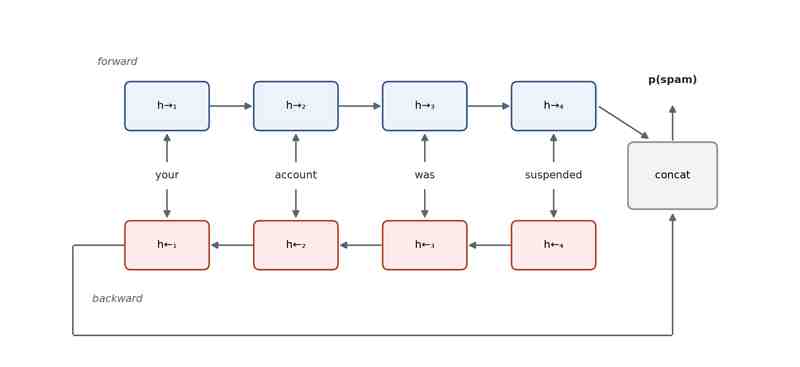
A left-to-right reader arrives at “your account was suspended” having accumulated context in one direction only; by the time it reaches “suspended” it has forgotten how the sentence opened. Schuster and Paliwal’s 1997 fix[12] is to run a second recurrence backwards and concatenate the two final states.
class Bi_LSTM_Classifier(_Recurrent_Base):
    """Reads forward and backward, then concatenates the two final states."""

    def __init__(self, vocab_size):
        super().__init__(vocab_size=vocab_size, head_in=2 * config.HIDDEN_DIM)
        self.core = nn.LSTM(
            config.EMBED_DIM, config.HIDDEN_DIM,
            num_layers=config.NUM_LAYERS, batch_first=True, bidirectional=True,
        )

    def forward(self, x, lengths):
        _, (hidden, _) = self.core(_pack(embedded=self.embedding(x), lengths=lengths))
        features = torch.cat((hidden[-2], hidden[-1]), dim=-1)
        return self.classify(features=features)
Line 82 is where the classifier head doubles to 256 inputs, because line 85 turns on the second direction. Line 90 is the concatenation worth reading closely: hidden[-2] is the forward direction’s last state and hidden[-1] the backward direction’s. Both are the state after that direction’s final real token, because line 89 packed the sequence first.
This is legitimate here and illegitimate in next-token prediction. Spam classification sees the whole message at once; there is no future to leak.
It is also, on this corpus, the best recurrent model. It reaches its best validation F1 at epoch 4 — faster than any other, because the backward pass gives the first tokens a short path to the output instead of a 200-step one.
7. Attention pooling
Every model so far throws away 199 hidden states and classifies from the last one. Bahdanau, Cho and Bengio’s 2015 alternative[13] is to keep all of them and learn a weighted average.
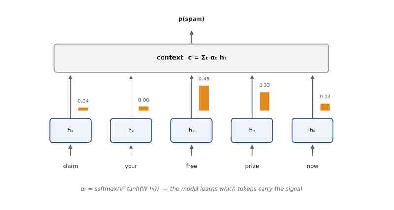
ut = tanh( W ht + b )

αt = exp( v⊤ ut ) / ∑k exp( v⊤ uk )

c = ∑t αt ht
A single learned query vector v scores each position; a softmax turns the scores into weights that sum to one; the context vector c is the weighted average, and the classifier sees c instead of hT.
def attend(self, outputs, pad_mask):
    scores = self.query(torch.tanh(self.project(outputs))).squeeze(-1)
    scores = scores.masked_fill(pad_mask, torch.finfo(scores.dtype).min)
    weights = torch.softmax(scores, dim=1)
    context = torch.bmm(weights.unsqueeze(1), outputs).squeeze(1)
    return context, weights
Line 109 projects each hidden state down, squashes it, and scores it against the learned query. Line 110 is essential and easy to forget: it drives the score of every pad position to the most negative representable number, so that line 111’s softmax gives them zero weight instead of spending probability mass on padding. Line 112 is the weighted average, written as a batched matrix multiply. The whole mechanism costs 16,512 parameters — a 256→64 projection and a 64→1 query — on top of the BiLSTM’s 2,824,449.
Because the weights are just numbers, you can read them. Here is the trained model on the spam message from section 2:
p(spam) = 0.9827
  winner   0.6399
  claim    0.1903
  <url>    0.0959
  now      0.0255
  at       0.0217
  prize    0.0175
  your     0.0064
  <cur>    0.0028
Line 1 is the model’s output probability; lines 2–9 are the attention weights, one per token, sorted. Nearly two-thirds of the mass lands on line 2 and another fifth on line 3. The model has learned that this message is spam because of two words, and it will tell you which two. That is worth something no accuracy number gives you.
Now a ham message:
p(spam) = 0.0025
  <num>     0.4091      ← "12"
  <num>     0.3461      ← "30"
  at        0.0627
  for       0.0537
  still     0.0490
  tomorrow  0.0422
  lunch     0.0090
Lines 2–3 carry three-quarters of the mass between them, and both are the same placeholder — the two halves of “12:30”, split by the regex quirk from section 2. The model is not reasoning about the time of lunch. Absent any spam evidence it dumps attention on the highest-frequency token in the vocabulary, and <num> — 339,172 occurrences — is exactly that. Attention weights are a diagnostic, not an explanation, and this is what the difference looks like.
8. Training
Every model shares the same skeleton — nn.Embedding → recurrent core → dropout[14] → nn.Linear(·, 1) — and the same recipe: Adam[15] at 1e-3, batch size 128, gradient clipping at norm 5.0, BCEWithLogitsLoss on a raw logit, up to 30 epochs, early stopping on validation F1 with patience 4.
Gradient clipping earns its place, though less dramatically than the folklore claims. Vanishing and exploding gradients are the same phenomenon with the spectral radius of Whh on either side of 1, and the vanilla RNN does spike: across three epochs its pre-clip gradient norm reaches 79.3, nearly sixteen times the clip threshold — though the median batch sits at 0.88 and only 2.9% of batches are clipped at all. Remove the clip and the norm reaches 101.3. It does not diverge — I ran it, and the loss stays finite — but it learns measurably worse, ending three epochs at a training loss of 0.477 against 0.253 with the clip in place, and its training loss climbs from epoch 2 to epoch 3 instead of falling. “Your RNN will NaN without clipping” is a claim worth testing before repeating; on this task it is false, and the clip is still worth having.
| Model | Parameters | Recurrent core | Best epoch | Epochs run | Best val F1 | Sec/epoch |
|---|---|---|---|---|---|---|
| Simple RNN | 2,593,153 | 33,024 | 9 | 13 | 0.9199 | 11.2 |
| LSTM | 2,692,225 | 132,096 | 20 | 24 | 0.9634 | 11.4 |
| GRU | 2,659,201 | 99,072 | 10 | 14 | 0.9655 | 11.3 |
| BiLSTM | 2,824,449 | 264,192 | 4 | 8 | 0.9674 | 14.8 |
| BiLSTM + attention | 2,840,961 | 280,704 | 5 | 9 | 0.9669 | 22.5 |
The parameter counts are dominated by something that has nothing to do with the architecture: the embedding table is 20,000 × 128 = 2,560,000 weights, which is 98.7% of the vanilla RNN and 90.1% of the attention model. The interesting part of each model — the recurrent core — is between 33 thousand and 281 thousand parameters. All five are, structurally, an embedding table with a small machine bolted on the end.
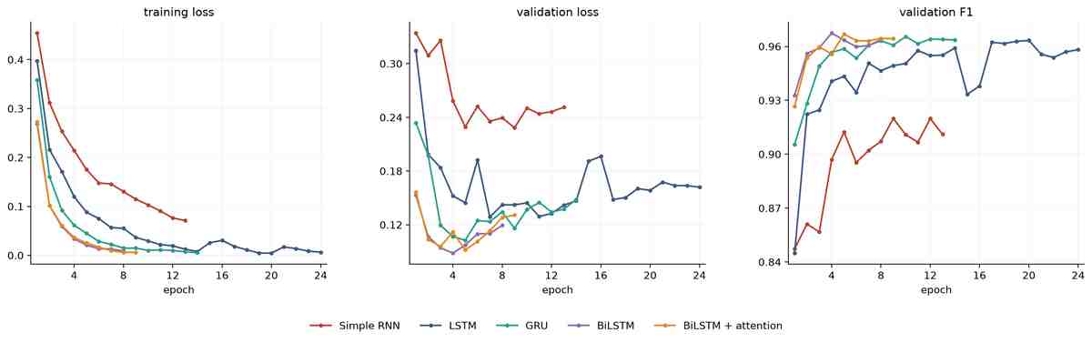
The middle panel of Fig 3 is the one to look at. For the LSTM and the GRU, validation loss bottoms out long before validation F1 peaks. The LSTM’s loss is lowest at epoch 7 (0.129) and drifts up to 0.158 by epoch 20 — while over exactly that stretch its F1 climbs from 0.951 to its peak of 0.963. The GRU does the same thing, loss bottoming at epoch 5 and F1 peaking at epoch 10.
The models are not getting more wrong. They are getting more confident about the handful of things they already have wrong, and cross-entropy punishes that much harder than F1 does. Early-stopping on validation loss would have halted the LSTM at epoch 7 and cost it 1.2 points of F1. (For the vanilla RNN, the BiLSTM, and the attention model the two criteria coincide — the loss minimum and the F1 peak land on the same epoch — which is exactly why you cannot check this on one model and assume it generalizes.)
The LSTM is the odd one out, taking 20 epochs to reach a best F1 that the BiLSTM reaches in 4. Same cell, same data; the only difference is that the bidirectional model gives early tokens a short path to the loss. It is the vanishing gradient again, showing up as an optimization speed rather than as a final score.
The whole suite trains in about 15 minutes on an RTX 3060 laptop GPU.
9. Results
Held-out test split: 3,972 messages, 41.9% spam, decision threshold 0.50.
| Model | Accuracy | Precision | Recall | F1 | FP | FN | ROC-AUC | PR-AUC |
|---|---|---|---|---|---|---|---|---|
| Simple RNN | 0.9403 | 0.9127 | 0.9483 | 0.9302 | 151 | 86 | 0.9760 | 0.9657 |
| LSTM | 0.9726 | 0.9659 | 0.9688 | 0.9673 | 57 | 52 | 0.9931 | 0.9905 |
| GRU | 0.9743 | 0.9716 | 0.9670 | 0.9693 | 47 | 55 | 0.9956 | 0.9934 |
| BiLSTM | 0.9776 | 0.9719 | 0.9748 | 0.9733 | 47 | 42 | 0.9963 | 0.9955 |
| BiLSTM + attention | 0.9741 | 0.9762 | 0.9616 | 0.9688 | 39 | 64 | 0.9960 | 0.9952 |
| TF-IDF + LogReg | 0.9821 | 0.9848 | 0.9724 | 0.9785 | 25 | 46 | 0.9984 | 0.9979 |
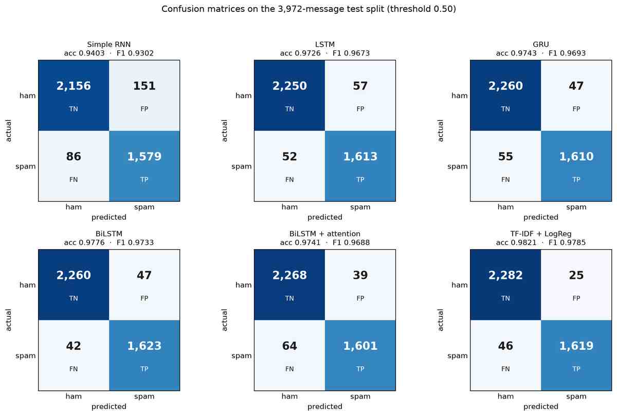
The architectural story lands exactly as advertised, and Fig 4 shows where each model spends its errors. Gating buys 3.7 points of F1 over the vanilla RNN. Bidirectionality buys another 0.6 on top of the LSTM. And then a linear model over TF-IDF n-grams beats all five.
I would not read much into the ordering among the gated models. GRU 0.9693, attention 0.9688, LSTM 0.9673 — these are single runs at a single seed (1337), and gaps of two or three thousandths of an F1 point are inside the noise you would get by changing the seed. The gaps that survive are RNN << gated << baseline.
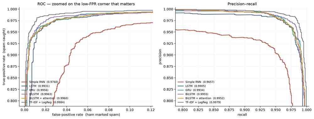
The zoom in Fig 5 is not cosmetic: it is the only region of the curve a deployed filter ever operates in, and section 11 is about what happens there. Per-source F1, meanwhile, shows where the difficulty actually lives:
| Model | UCI SMS | SpamAssassin | Enron |
|---|---|---|---|
| Simple RNN | 0.6842 | 0.8421 | 0.9549 |
| LSTM | 0.7338 | 0.9667 | 0.9788 |
| GRU | 0.7218 | 0.9663 | 0.9813 |
| BiLSTM | 0.8030 | 0.9602 | 0.9828 |
| BiLSTM + attention | 0.7360 | 0.9605 | 0.9802 |
| TF-IDF + LogReg | 0.8430 | 0.9745 | 0.9848 |
Every model is 10 to 25 points worse on SMS than on Enron. SMS is 508 of the 3,972 test messages and only 58 of them are spam, so the models are optimizing a loss that barely notices SMS at all — Enron contributes 72% of the test set and 86% of the spam. The mixed corpus makes the evaluation honest and the training harder, which is the trade it was chosen for. The vanilla RNN’s SMS F1 of 0.684 is the clearest single indictment of it in this whole article.
10. Why the linear model wins
Spam is a bag-of-phrases problem. “Viagra”, “click here”, “your account has been suspended” — the vocabulary is the signal, and word order carries far less of it than a sequence model is built to extract. The RNNs spend their capacity learning an ordering structure the task does not reward.
But three concrete asymmetries matter more than that hand-wave, and two of them favour the baseline.
The baseline reads the whole message. TfidfVectorizer sees every token of every e-mail. The recurrent models see the first 200 and nothing else — which, as established, is 28.3% of training messages truncated for the neural models and 0% for the baseline. This is not a fair fight, and it is not fair in the direction the headline suggests. Raising MAX_SEQ_LEN is the first experiment anyone should run against this result.
The baseline has five times the lexical capacity. 100,000 n-gram features — 23,607 unigrams and 76,393 bigrams — against a 20,000-token vocabulary. And those 76,393 bigrams give the linear model exactly the amount of word-order sensitivity spam actually needs (click here, call phone, for you) without any of the machinery.
The two models do not see identical tokens. scikit-learn’s[16] default token_pattern, (?u)\b\w\w+\b, strips the angle brackets and drops single-character tokens, so the baseline’s <num> is num and it never sees a or i at all. A small difference, but it means “the same masked text” is not quite the same input.
Now the part that should bother you. Here are the strongest coefficients in each direction:
| Strongest spam evidence | Weight | Strongest ham evidence | Weight |
|---|---|---|---|
| http | +12.38 | enron | −17.51 |
| your | +10.34 | vince | −8.44 |
| remove | +8.06 | wrote | −8.06 |
| our | +7.88 | url date | −7.66 |
| software | +7.68 | attached | −6.96 |
| viagra | +7.60 | url url | −6.94 |
| here | +7.57 | louise | −6.73 |
| goodbye | +6.82 | enron com | −6.66 |
| re num | +6.79 | gas | −5.81 |
| cur | +6.67 | houston | −5.51 |
| online | +6.53 | thanks | −5.21 |
| call phone | +5.89 | ect | −4.99 |
| mobile | +5.60 | energy | −4.62 |
| paliourg | +5.20 | that | −4.59 |
The single largest coefficient in the entire model, in either direction, is enron at −17.51. Larger than http. Larger than viagra. Following it: vince (Vince Kaminski, an Enron employee whose mailbox is in the corpus), louise (Louise Kitchen, likewise), houston, gas, energy, ect (Enron Capital & Trade). And paliourg on the spam side is not a spam word at all — it is Georgios Paliouras, one of the researchers who published the corpus, whose name leaked into the spam files.
None of this is spam detection. The model has discovered that mail about the natural gas business in Houston is ham, and it has discovered it so effectively that “Enron” outweighs “Viagra”. The ham in these corpora is not neutral: SpamAssassin’s is Linux and developer mailing-list traffic, Enron’s is intra-company mail. A classifier can score 98% by learning topic, and this one demonstrably does, at least in part.
Which reframes the headline. The baseline does not beat the RNNs because linear models are secretly better at language. It beats them because it is a more efficient memorizer of the corpus’s idiosyncrasies, and it was handed the whole message to memorize while the RNNs were handed the first 200 tokens. The right conclusion is not “don’t use RNNs for spam” — it is “this benchmark is measuring less than it appears to, and a strong baseline is how you find that out.” Skipping the TF-IDF run would have left me with a tidy 97.8% BiLSTM and no idea that enron was doing the work.
11. The threshold you actually ship
Every number above uses a decision threshold of 0.50, which is a number nobody in production has ever chosen on purpose. It weights a false positive — a real message dropped in the spam folder, a missed invoice, a missed job offer — exactly as much as a false negative, which is one more piece of junk the user deletes in a second. The real cost ratio is not 1:1. It is closer to 1:1000.
So src/evaluate.py reports every model twice: once at 0.50, and once at a threshold chosen on the validation split to hold the FPR at or under TARGET_MAX_FPR = 0.001. The threshold is picked on validation and applied to test, which is the only way the number means anything.
The trade is brutal:
| Model | Threshold | Recall | Precision | FP | Test FPR |
|---|---|---|---|---|---|
| Simple RNN | 0.9947 | 23.6% | 0.9874 | 5 | 0.0022 |
| LSTM | 0.99991 | 48.7% | 0.9939 | 5 | 0.0022 |
| GRU | 0.99991 | 59.5% | 0.9970 | 3 | 0.0013 |
| BiLSTM | 0.99938 | 61.8% | 0.9990 | 1 | 0.0004 |
| BiLSTM + attention | 0.99932 | 63.5% | 0.9991 | 1 | 0.0004 |
| TF-IDF + LogReg | 0.98214 | 60.3% | 1.0000 | 0 | 0.0000 |
Two things happen here, and both are invisible at 0.50.
First, everything collapses. The BiLSTM goes from catching 97.5% of spam to catching 61.8% of it. If you promise a user that you will misfile at most one legitimate message in a thousand, you are promising to let through nearly 40% of their spam. That is the actual product decision, and no accuracy table shows it to you.
Second, the ranking changes. The attention model is fourth on accuracy at 0.50 — behind the baseline, the BiLSTM, and the GRU. Under the false-positive budget it catches more spam than any other model, including the baseline. Its high-confidence tail is better calibrated: it is right when it is certain. Attention pooling never looked worth its 16,512 parameters in the headline table, and in the only regime that resembles deployment it is the best model in the study.
The baseline, meanwhile, achieves zero false positives on the test split at its tuned threshold, and pays about three points of recall for it.
Reporting accuracy alone would have hidden every word of this.
12. What this experiment does not show
- One seed. SEED = 1337, one run per model, no error bars. Differences below roughly half an F1 point should be treated as noise.
- Best-checkpoint comparison. Each model early-stops on its own best validation F1, so the table compares each architecture’s best epoch, not a fixed epoch budget. The LSTM needed 20 epochs; the BiLSTM needed 4.
- The truncation asymmetry is unresolved. 200 tokens for the RNNs, unlimited for the baseline. Until that is equalized, the headline comparison overstates the baseline’s advantage by an unknown amount.
- Topic leakage is real and unquantified. The enron coefficient proves the models can classify on subject matter. Per-source metrics contain it; they do not eliminate it. The honest fix is a fourth corpus of ham from a completely different domain.
- No pretrained embeddings, no transformer. The embedding table is learned from scratch on 31,771 messages. A fine-tuned DistilBERT would very likely beat everything here, and would also cost more than 15 minutes on a laptop GPU.
- <num> is doing too much work. 339,172 occurrences of a single placeholder, and an attention model that dumps 75% of its mass onto it when it has nothing better to say. Splitting it — years, prices, quantities, short numeric codes — is an obvious improvement nobody has tried here.
Reproducing this
python -m venv .venv
.venv\Scripts\activate          # Windows;  source .venv/bin/activate elsewhere
pip install -r requirements.txt

python src/download_data.py     # fetch the three corpora into data/raw/
python src/build_dataset.py     # parse, de-duplicate, stratified split
python src/train_all.py         # five RNNs + the TF-IDF baseline
python src/evaluate.py          # confusion matrices, both thresholds -> results/metrics.json

python src/predict.py --text "WINNER!! Claim your free prize now"
Lines 1–3 create the virtual environment and install the pinned dependencies. Lines 5–8 are the pipeline in order: fetch, build, train, evaluate — each one reads what the previous wrote, so they run once and in sequence. Line 10 scores a single message against the trained checkpoint, which is the fastest way to confirm the whole chain works.
Every tunable — paths, dataset URLs, sequence length, vocabulary size, hidden width, learning rate, early-stopping patience, the false-positive budget — lives in config.py, and nothing is hard-coded anywhere else. Changing MAX_SEQ_LEN and rerunning is a twenty-minute experiment, and it is the first one I would run.
Key takeaways
- A vanilla RNN on a 200-token e-mail depends on roughly its last eight tokens, and the gradient reaching token 1 is exactly zero in float32. Gradients and occlusion agree, so this is a property of the model rather than of one measurement.
- Gating is what buys the memory: 3.7 points of F1 over the vanilla RNN, and a gradient that decays by a factor of 15 (GRU) rather than by underflow.
- A TF-IDF logistic regression beat all five recurrent models — but it read whole messages while the RNNs read 200 tokens, so the benchmark, not the architecture, decided a large part of that.
- The largest coefficient in that linear model is enron, not viagra. A strong, inspectable baseline is how topic leakage becomes visible at all.
- At a deployable false-positive budget of one in a thousand, every model loses a third to three-quarters of its recall, and the ranking reorders. Accuracy at threshold 0.50 hides this completely.
- Validation loss and validation F1 peak at different epochs for the LSTM and the GRU, so the early-stopping criterion is a modelling decision, not a detail.
The complete, runnable code for every figure above lives in the companion repository under src/. Full attribution for every dataset and library is in the repository’s RESOURCES.md. The corpora are fetched at run time into a git-ignored data/ directory; nothing is redistributed here.
Resources
Every asset, dataset, and library cited above — numbered in order of first appearance. Sample assets are used under the license noted for each; the derived images in this article are derivative works of them. Click any bracketed marker such as [1] to jump to its entry.
- [1] Finding Structure in Time — Elman, Cognitive Science 14(2), 1990. doi.org/10.1207/s15516709cog1402_1
- [2] SMS Spam Collection v.1 — Almeida, Gómez Hidalgo & Yamakami, DOCENG 2011. CC BY 4.0. archive.ics.uci.edu/dataset/228
- [3] SpamAssassin public corpus — Apache SpamAssassin Project, 2003 & 2005. Freely redistributable for research; the SpamAssassin software itself is Apache-2.0. spamassassin.apache.org/old/publiccorpus
- [4] Enron-Spam — Metsis, Androutsopoulos & Paliouras, CEAS 2006. The single-CSV mirror used here is packaged GPL-3.0, which covers the packaging and build script rather than the underlying research corpus; anyone republishing the messages should return to the original release terms. github.com/MWiechmann/enron_spam_data
- [5] PyTorch — Paszke et al., PyTorch: An Imperative Style, High-Performance Deep Learning Library, NeurIPS 2019. BSD-3-Clause. pytorch.org
- [6] Untersuchungen zu dynamischen neuronalen Netzen — Hochreiter, diploma thesis, TU München, 1991. The vanishing gradient. people.idsia.ch/~juergen
- [7] Learning long-term dependencies with gradient descent is difficult — Bengio, Simard & Frasconi, IEEE Transactions on Neural Networks 5(2), 1994. doi.org/10.1109/72.279181
- [8] Long Short-Term Memory — Hochreiter & Schmidhuber, Neural Computation 9(8), 1997. doi.org/10.1162/neco.1997.9.8.1735
- [9] Learning to Forget: Continual Prediction with LSTM — Gers, Schmidhuber & Cummins, Neural Computation 12(10), 2000. The forget gate. doi.org/10.1162/089976600300015015
- [10] Learning Phrase Representations using RNN Encoder–Decoder for Statistical Machine Translation — Cho et al., EMNLP 2014. The GRU. arxiv.org/abs/1406.1078
- [11] Empirical Evaluation of Gated Recurrent Neural Networks on Sequence Modeling — Chung, Gulcehre, Cho & Bengio, 2014. arxiv.org/abs/1412.3555
- [12] Bidirectional Recurrent Neural Networks — Schuster & Paliwal, IEEE Transactions on Signal Processing 45(11), 1997. doi.org/10.1109/78.650093
- [13] Neural Machine Translation by Jointly Learning to Align and Translate — Bahdanau, Cho & Bengio, ICLR 2015. Attention. arxiv.org/abs/1409.0473
- [14] Dropout: A Simple Way to Prevent Neural Networks from Overfitting — Srivastava, Hinton, Krizhevsky, Sutskever & Salakhutdinov, JMLR 15, 2014. jmlr.org/papers/v15/srivastava14a.html
- [15] Adam: A Method for Stochastic Optimization — Kingma & Ba, ICLR 2015. arxiv.org/abs/1412.6980
- [16] scikit-learn — Pedregosa et al., Scikit-learn: Machine Learning in Python, JMLR 12, 2011. BSD-3-Clause. scikit-learn.org