A hand-held phone shot of a face at dusk comes back tiny, tilted, smeared by a shaky hand and freckled with sensor noise — and yet a network with fewer parameters than a spreadsheet has cells can walk most of that damage back. This article builds that network end to end: it takes a common face dataset, shrinks and wrecks every picture to imitate a bad low-light capture, and trains the classic three-layer SR network to reconstruct the sharp original — on a laptop, with no GPU required.
Code: github.com/babak-abad/Super_Resolution
The problem, and the plan
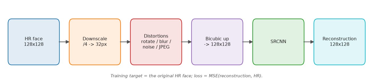
Single-image super-resolution is the task of turning one small, degraded picture back into a larger, sharp one. It is under-determined — many high-resolution scenes could have produced the same blurry thumbnail — so a model has to learn what faces usually look like and hallucinate the missing detail plausibly. To train such a model we need pairs: a clean HR face and a matching wrecked LR version. We manufacture those pairs by taking sharp faces and degrading them ourselves, which means we always know the ground truth. The whole pipeline is a short assembly line, shown in Fig 1.
Getting the data
For faces we use LFW (Labeled Faces in the Wild)[1], a classic, easy-to-fetch collection of everyday photographs of faces. The loader from scikit-learn[2] downloads and caches it on the first run, so src/download_data.py just has to take a centred square crop of each face and resize it to a uniform 128×128 — that square is our high-resolution ground truth. Point the same script at any other folder of images instead (a single setting, covered at the end) and it builds the pool from those, which is what makes the project reusable on your own photos.
Simulating a noisy low-resolution shot
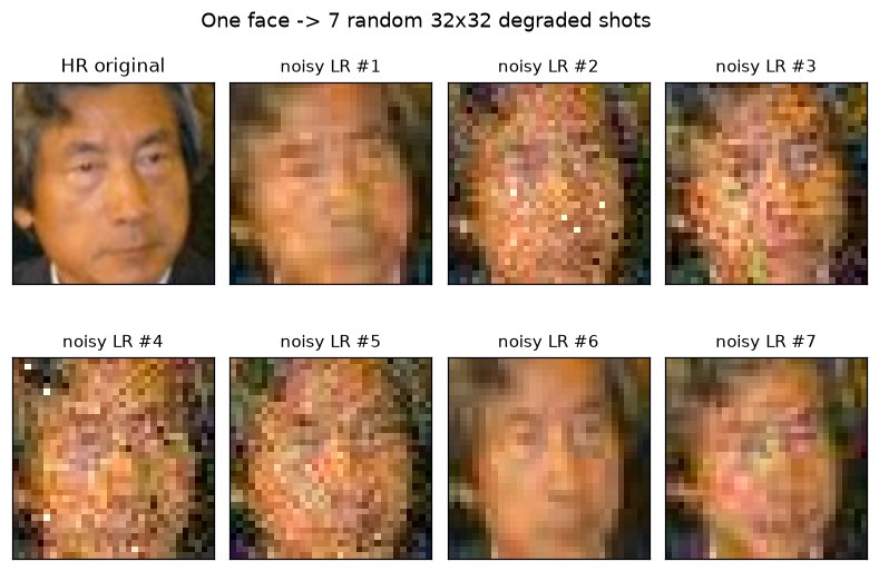
A believable low-resolution image is not just a shrunk one: a real capture also suffers a small rotation from an unsteady hand, motion blur, a little zoom in or out, sensor noise, salt-and-pepper dropouts, and JPEG compression when it is saved. Rather than hand-code each effect, we chain them with Albumentations[3], an image-augmentation library whose warps and resizes run on OpenCV[4]. One Compose expresses the whole capture.
import albumentations as A
import cv2

def build_degrade_pipeline():
    return A.Compose([
        A.Rotate(limit=8, border_mode=cv2.BORDER_REFLECT_101, p=0.9),
        A.Affine(scale=(0.9, 1.1), border_mode=cv2.BORDER_REFLECT_101, p=0.9),
        A.MotionBlur(blur_limit=7, p=0.9),
        A.Resize(height=32, width=32, interpolation=cv2.INTER_AREA),
        A.GaussNoise(std_range=(0.02, 0.12), p=0.9),
        A.SaltAndPepper(amount=(0.0, 0.02), p=0.9),
        A.ImageCompression(quality_range=(40, 80), p=0.9),
    ])
Line 5 opens the pipeline; lines 6–8 apply the capture-resolution effects — a small Rotate, an Affine scale that zooms in or out, and MotionBlur. Line 9 is the key step: it downscales the 128×128 face to the 32×32 sensor with area interpolation. Lines 10–12 then dirty that small image the way a sensor and file format would — Gaussian noise, salt & pepper, and JPEG. Every draw is random (each has probability p=0.9), so the same face yields a different shot each time; the literal limits shown here live in config.py in the repository. The result is the variety in Fig 2.
Pairing low- and high-resolution
SRCNN expects its input at the target size: it sharpens an image, it does not enlarge one. So each 32×32 shot is bicubic-upsampled back to 128×128 before it reaches the network — a blurry, full-size starting point the model will clean up. A small PyTorch[5] Dataset ties each upsampled input to its clean target.
def _bicubic_upsample(lr_image):
    return cv2.resize(lr_image, (128, 128), interpolation=cv2.INTER_CUBIC)

class Sr_Dataset(torch.utils.data.Dataset):
    def __init__(self, hr_paths, augment):
        self.hr_paths = list(hr_paths)
        self.augment = augment
        self.pipeline = build_degrade_pipeline()

    def __getitem__(self, index):
        hr = self.load_hr(index)
        lr_up = _bicubic_upsample(self.make_lr(index, hr))
        return image_to_tensor(lr_up), image_to_tensor(hr)
Lines 1–2 do the bicubic enlargement back to 128×128. Line 8 builds the degradation pipeline once per dataset and reuses it. The heart is __getitem__ on lines 10–13: line 11 loads the clean HR face, line 12 degrades it to a small noisy shot and upsamples that back to full size, and line 13 returns the pair (blurry input, sharp target) as tensors. Because the degradation is redrawn on every access, the network effectively never sees the same training example twice. Validation faces are degraded with a fixed seed so their scores are comparable across epochs.
The model: three convolutions
The reconstructor is SRCNN[6], the network that launched deep-learning super-resolution in 2014. It is just three convolutions and famously easy to read: extract patches, map them non-linearly, then reconstruct.
import torch.nn as nn

class Sr_Cnn(nn.Module):
    def __init__(self, num_channels=3):
        super().__init__()
        self.features = nn.Sequential(
            nn.Conv2d(num_channels, 64, kernel_size=9, padding=4),
            nn.ReLU(inplace=True),
            nn.Conv2d(64, 32, kernel_size=5, padding=2),
            nn.ReLU(inplace=True),
            nn.Conv2d(32, num_channels, kernel_size=5, padding=2),
        )

    def forward(self, x):
        return self.features(x)
Line 7 is the 9×9 patch-extraction layer that lifts the 3 colour channels to 64 feature maps; line 9 is the 5×5 non-linear mapping down to 32 maps; line 11 is the 5×5 reconstruction back to 3 channels. Every convolution is padded so the image stays 128×128 from input to output, and the ReLUs on lines 8 and 10 supply the non-linearity. That is the entire model — just 69,251 learnable parameters, small enough to train comfortably on a CPU. Training minimises the MSE between the reconstruction and the true HR face, and we track quality with PSNR[7]:
MSE = (1 / N) ∑i (xi − yi)² PSNR = 10 · log10( 1 / MSE ) dB
Training
With pairs and a model in hand, the loop is textbook: an Adam optimiser, MSE loss, and a per-epoch check of validation PSNR so we can keep the best weights.
model = Sr_Cnn().to(device)
criterion = nn.MSELoss()
optimizer = torch.optim.Adam(model.parameters(), lr=1e-3)

for epoch in range(1, EPOCHS + 1):
    model.train()
    for lr_up, hr in train_loader:
        lr_up, hr = lr_up.to(device), hr.to(device)
        optimizer.zero_grad()
        loss = criterion(model(lr_up), hr)
        loss.backward()
        optimizer.step()
    val_psnr, bicubic_psnr = evaluate(model=model, loader=val_loader, device=device)
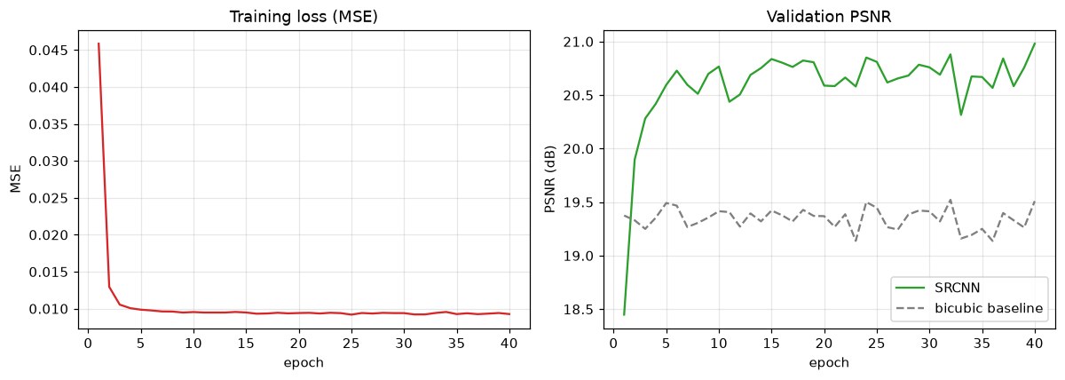
Lines 1–3 build the model, the MSE loss, and the Adam optimiser. The epoch loop starts on line 5; the batch loop on line 7 moves each pair to the device. Line 10 is where learning happens: the network reconstructs lr_up and the loss compares it to the sharp target hr; lines 11–12 backpropagate and step. Line 13 evaluates validation PSNR against the plain bicubic baseline each epoch — the same comparison plotted in Fig 3. Running src/train.py saves the best weights to checkpoints/ and the full history to results/metrics.json.
Results
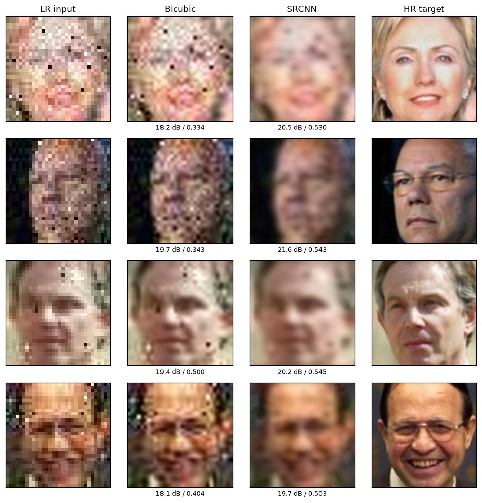
On the held-out validation faces, SRCNN beats the bicubic starting point on both PSNR and SSIM[7] (the latter computed with scikit-image[8]). The numbers below are averaged over the whole validation split.
| Metric | Bicubic input | SRCNN |
|---|---|---|
| PSNR (dB) | 19.17 | 20.61 |
| SSIM | 0.441 | 0.560 |
The visual difference in Fig 4 is clearer than the decibels suggest: SRCNN removes the speckle, tightens edges around the eyes and mouth, and recovers a face that reads as a real person rather than a smear. It will not invent detail that the small input never contained — no method can — but it consistently improves on the bicubic guess. The montage is written by src/reconstruct.py using Matplotlib[9].
When one shot isn’t enough: multi-frame super-resolution
SRCNN only ever sees the single frame it is handed, so any detail that frame lost it has to invent from what faces usually look like. But a phone rarely takes just one picture — a burst of shots of the same face arrives a few milliseconds apart, each with slightly different hand-shake, blur and sensor noise. MFSR (multi-frame super-resolution) exploits exactly that: because every shot samples the scene on a slightly shifted pixel grid, several noisy low-resolution frames together carry more real information than any one of them. The idea is decades old — robust multi-frame reconstruction goes back to classical work[10] — and a modern version is what powers the “Super Res Zoom” on today’s phone cameras[11].
Where single-image super-resolution (SISR) leans entirely on learned priors, MFSR also has real, complementary measurements to fuse. The two tasks differ only in what enters the network:
| Aspect | Single-image (SISR) | Multi-frame (MFSR) |
|---|---|---|
| Input | one degraded shot — 3 channels | N stacked shots — 3×N channels |
| Model | Sr_Cnn | Sr_Cnn_Mf — early fusion; only the first 9×9 conv widens |
| Parameters (N = 5) | 69,251 | 131,459 |
| Missing detail comes from | learned face priors only | priors plus sub-pixel detail spread across frames |
| Sensor noise | must be removed from one frame | independent per frame, so it averages down |
| Ideal when | only one photo exists | several shots of one near-static scene exist |
Fusing the frames: a multi-frame SRCNN
The change to the model is deliberately tiny, so the comparison stays honest. We stack the N upsampled shots on the channel axis and let a single widened first convolution fuse them — everything downstream is the original SRCNN.
import torch.nn as nn

class Sr_Cnn_Mf(nn.Module):
    def __init__(self, num_channels=3, num_frames=5):
        super().__init__()
        self.features = nn.Sequential(
            nn.Conv2d(num_channels * num_frames, 64, kernel_size=9, padding=4),
            nn.ReLU(inplace=True),
            nn.Conv2d(64, 32, kernel_size=5, padding=2),
            nn.ReLU(inplace=True),
            nn.Conv2d(32, num_channels, kernel_size=5, padding=2),
        )

    def forward(self, x):
        return self.features(x)
Only line 7 differs from the single-image network: the first 9×9 convolution now accepts num_channels * num_frames input channels — 15 for the default five-frame model — and fuses every frame in that very first layer (early fusion). Lines 9 and 11, the 5×5 mapping and the 5×5 reconstruction, are identical to Sr_Cnn, so any gain comes purely from having more frames to look at, not from a heavier head. What feeds this model is built in the dataset by stacking the shots:
def __getitem__(self, index):
    hr = self.load_hr(index)
    frames = self.make_lr_frames(index, hr)
    stack = torch.cat(
        [image_to_tensor(_bicubic_upsample(f)) for f in frames], dim=0
    )
    return stack, image_to_tensor(hr)
Line 2 loads the clean HR face and line 3 degrades it into num_frames independent shots — each with its own random rotation, blur and noise, exactly the variety in Fig 2. Lines 4–6 bicubic-upsample every shot back to 128×128 and concatenate them along the channel axis (dim=0) into one 15×128×128 tensor; line 7 pairs that stack with the sharp target. Each shot is seeded per face and frame, so shot k of a validation face is identical whether the model fuses two frames or seven — adding frames only appends new views, which is what makes the frame sweep a fair test.
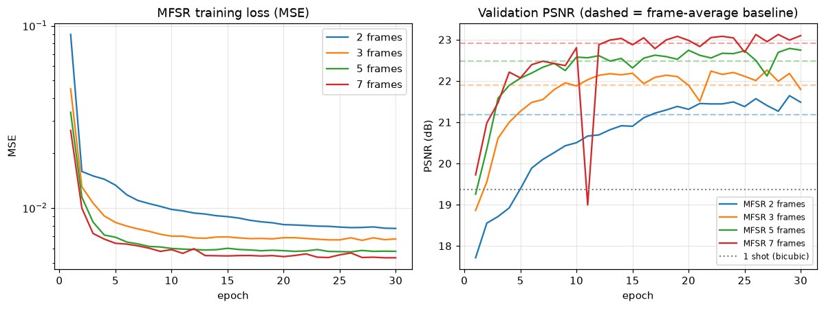
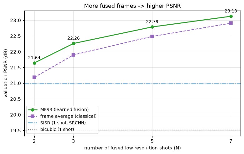
Training is otherwise unchanged — same Adam, same MSE loss, same per-epoch PSNR check. Running src/train_mfsr.py trains one model for each of N ∈ {2, 3, 5, 7} fused frames and writes the full sweep to results/mfsr_metrics.json, tracking two baselines every epoch: a single upsampled shot (where SISR starts) and the plain pixel-wise average of the N shots (classical fusion with no learning). Fig 5 shows every model converging, and Fig 6 distils the sweep into one trend: more frames, higher PSNR — and the learned fusion stays above the plain average at every frame count.
Single-frame vs multi-frame, head to head
To compare the two approaches fairly we score them on the same shots: the single-image model reconstructs from frame 1, while the five-frame model additionally sees frames 2–5 of the identical face. Averaged over the whole validation split:
| Method | Frames | PSNR (dB) | SSIM |
|---|---|---|---|
| Bicubic (one shot) | 1 | 19.25 | 0.444 |
| SISR — SRCNN | 1 | 20.72 | 0.563 |
| Frame average | 5 | 22.61 | 0.599 |
| MFSR — learned fusion | 5 | 22.93 | 0.638 |
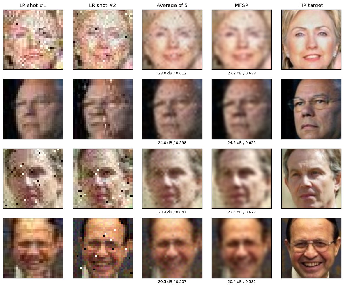
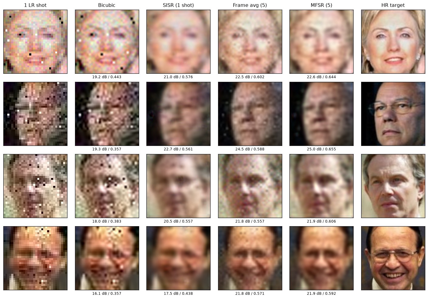
The jump from SISR to MFSR is about 2.2 dB — far larger than the gain SISR itself won over bicubic — because the extra frames supply real detail instead of a learned guess. Fusion also beats the naive average, most clearly on SSIM (0.638 vs 0.599): a plain average cancels the independent sensor noise but smears edges, whereas the network learns to average the noise and keep the structure sharp. Fig 7 shows the fused output beside the frames and their average, and Fig 8 puts all four methods on the same faces — quality rises left to right, and MFSR takes the highest SSIM on every row.
Reusing it on your own images
Nothing above is face-specific. Every tunable lives in config.py, so to super-resolve your own photos you point INPUT_DIR at a folder and rerun the same two commands — the pipeline lowers your images, pairs them, and retrains with no code changes.
# config.py
INPUT_DIR = r"D:\my_photos"   # any folder tree of images
HR_SIZE = 128                 # target high-resolution size
SCALE = 4                     # downscale factor, so LR is 32 px
Line 2 switches the source from LFW to your folder; lines 3–4 set the target size and how aggressively to shrink it. Then rebuild and retrain:
python src/download_data.py
python src/train.py
python src/reconstruct.py
Line 1 rebuilds the HR pool from your folder, line 2 retrains SRCNN on it (using a GPU automatically when one is present), and line 3 writes the fresh comparison montage.
Key takeaways
- Super-resolution needs paired data; degrading sharp images yourself gives you unlimited pairs with perfect ground truth.
- A realistic degradation matters as much as the model — rotation, blur, noise, salt & pepper and JPEG, composed once with Albumentations, teach the network to denoise as well as sharpen.
- SRCNN’s three convolutions and 69,251 parameters are enough to beat a bicubic baseline on both PSNR and SSIM, and it trains on a CPU.
- Because every knob is in config.py, the same project retrains on any image folder — faces were just a convenient example.
- When several shots of one scene are available, fusing them (MFSR) beats a single-frame model by roughly 2 dB — the extra frames carry real detail and let independent sensor noise average out, and learned fusion still beats a plain average on structure (SSIM).
- For sharper results, swap SRCNN for a sub-pixel network such as ESPCN[12], which learns the upsampling itself instead of relying on bicubic.
The complete, runnable code for every figure above lives in the companion repository under src/. Full attribution for the dataset and every library is in the repository’s RESOURCES.md.
Resources
Every dataset, library, and method cited above — numbered in order of first appearance. The LFW photographs are used here for research/education under the terms noted below; the degraded and reconstructed images in this article are derivative works of them. Click any bracketed marker such as [1] to jump to its entry.
- [1] Labeled Faces in the Wild (LFW) — Huang, Ramesh, Berg, Learned-Miller, UMass Amherst TR 07-49, 2007; research/educational use, individual photo copyrights held by their owners. vis-www.cs.umass.edu/lfw
- [2] scikit-learn — Pedregosa et al., JMLR 2011, BSD-3-Clause; the LFW loader. scikit-learn.org
- [3] Albumentations — Buslaev et al., Information 2020, MIT; the degradation pipeline. albumentations.ai
- [4] OpenCV — Bradski, 2000, Apache-2.0; resize / warp backend. opencv.org
- [5] PyTorch — Paszke et al., NeurIPS 2019, BSD-3-Clause; model and training. pytorch.org
- [6] SRCNN — Dong, Loy, He, Tang, Image Super-Resolution Using Deep Convolutional Networks, IEEE TPAMI 2016. arxiv.org/abs/1501.00092
- [7] PSNR / SSIM — Wang, Bovik, Sheikh, Simoncelli, Image Quality Assessment: From Error Visibility to Structural Similarity, IEEE TIP 2004. doi.org/10.1109/TIP.2003.819861
- [8] scikit-image — van der Walt et al., PeerJ 2014, BSD-3-Clause; the SSIM metric. scikit-image.org
- [9] Matplotlib — Hunter, CiSE 2007, PSF-based license; the result figures. matplotlib.org
- [10] Multi-frame super-resolution — Farsiu, Robinson, Elad, Milanfar, Fast and Robust Multiframe Super Resolution, IEEE TIP 2004. doi.org/10.1109/TIP.2004.834669
- [11] Handheld Multi-Frame Super-Resolution — Wronski et al., ACM TOG (SIGGRAPH) 2019; the phone-camera “Super Res Zoom” pipeline. doi.org/10.1145/3306346.3323024
- [12] ESPCN — Shi et al., Real-Time Single Image and Video Super-Resolution Using an Efficient Sub-Pixel Convolutional Neural Network, CVPR 2016. arxiv.org/abs/1609.05158