YOLO V1

Before 2016, making a computer find every object in a photo meant running a classifier thousands of times across a sliding window, or first proposing a couple of thousand candidate regions and scoring each one. It worked, but it was slow and awkward. Then a paper with a memorable name changed the framing entirely: You Only Look Once^[1]. YOLO treats detection as a single regression problem — one network, one forward pass, straight from pixels to a grid of boxes and class scores. This article rebuilds YOLO v1 from scratch to explain exactly how that works: what the output tensor means, how a box becomes a row of numbers, and how one loss function ties classification and localisation together.

Code: github.com/babak-abad/YOLO-V1

What object detection actually asks

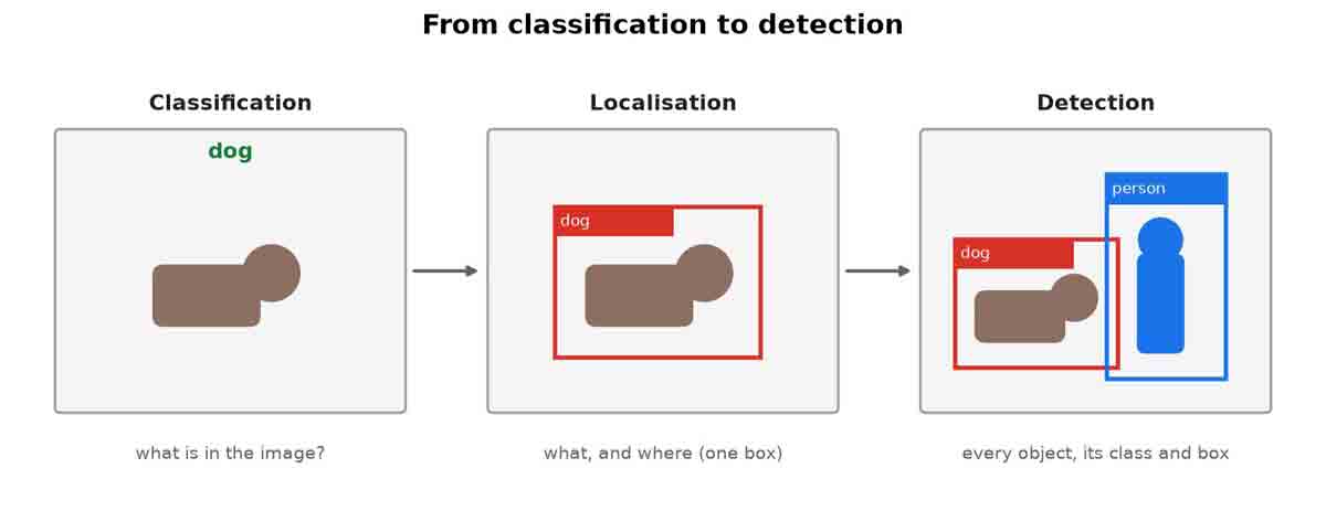
It helps to separate three tasks that are easy to confuse. Classification answers “what is in this image?” with a single label. Localisation goes further: name the main object and draw a box around it. Detection is the hard, general version — find every object, of any class, and give each one its own box, as in Fig 1. A detector therefore has to answer “how many, which classes, and where?” all at once, and the number of answers changes from image to image.

Two jobs at once: classification and regression

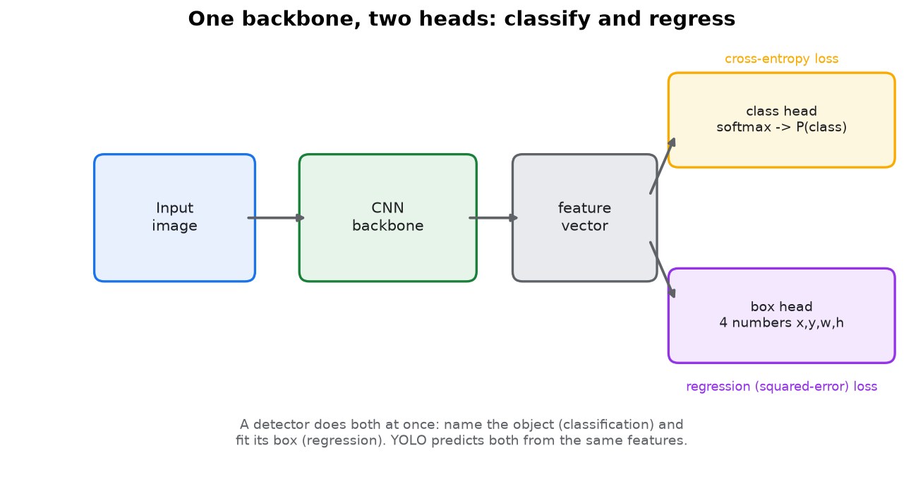
Every modern detector is really doing two things for each object it reports, shown in Fig 2. It classifies — a discrete choice over categories, trained with a cross-entropy-style loss — and it regresses a box, four continuous numbers (a centre, a width, a height) trained with a squared-error loss. Region-based methods like R-CNN^[2] bolt these two heads onto cropped region proposals. YOLO's insight is that both heads can read from the same feature map and produce all the answers for the whole image in one shot.

Where detectors came from: the sliding window

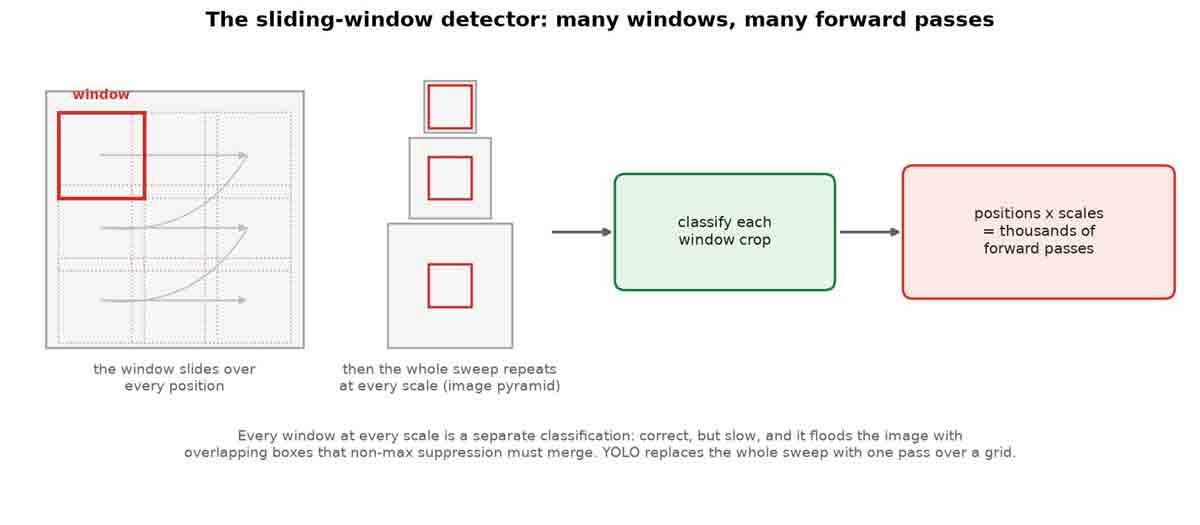
The oldest recipe for turning a classifier into a detector is the sliding window. Slide a fixed-size box across the image, crop the patch under it, and ask the classifier “is there an object here?”. Because objects come at different sizes, you repeat the whole sweep over an image pyramid — the image shrunk to several scales. The Viola–Jones face detector^[3] and, later, ConvNet detectors like OverFeat^[4] worked this way. Fig 3 shows the cost: positions × scales adds up to thousands of forward passes per image, and the overlapping positive windows then have to be merged by non-max suppression. It is correct but wasteful — the same convolutional features get recomputed again and again.

Anchors: giving each location a head start

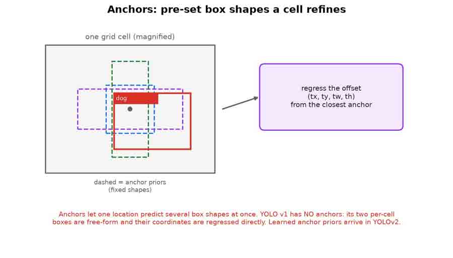
A refinement that region-proposal networks such as Faster R-CNN^[5] made popular is the anchor box. Instead of predicting a box from nothing, you attach a small set of pre-set reference shapes — tall, wide, big, small — to every location, and the network only has to predict a small offset that nudges the closest anchor onto the real object (Fig 4). Anchors let one location commit to several box shapes at once and make training more stable.

It is worth being precise here, because it is the one thing readers most often get wrong about YOLO v1: v1 has no anchors. Each of its grid cells predicts two boxes directly, as raw coordinates regressed through a fully-connected layer, with no learned prior shapes to refine. Learned anchor priors arrive one version later, in YOLOv2^[6], which removes v1's fully-connected layers precisely so it can predict offsets from anchors instead. Keeping that distinction straight is what makes the next section — reading v1's raw output — make sense.

Reading YOLO's output

Here is the whole idea in one picture. YOLO divides the input into an S × S grid (v1 uses S = 7). Each cell is responsible for the objects whose centre falls inside it, and each cell emits a fixed-length vector: B boxes, each with a confidence and four coordinates, plus C class probabilities shared across the whole cell. With v1's B = 2 boxes and C = 20 VOC classes that is 2 × 5 + 20 = 30 numbers per cell, so the full output is a 7 × 7 × 30 tensor — 1470 numbers produced in a single forward pass, laid out as in Fig 5.

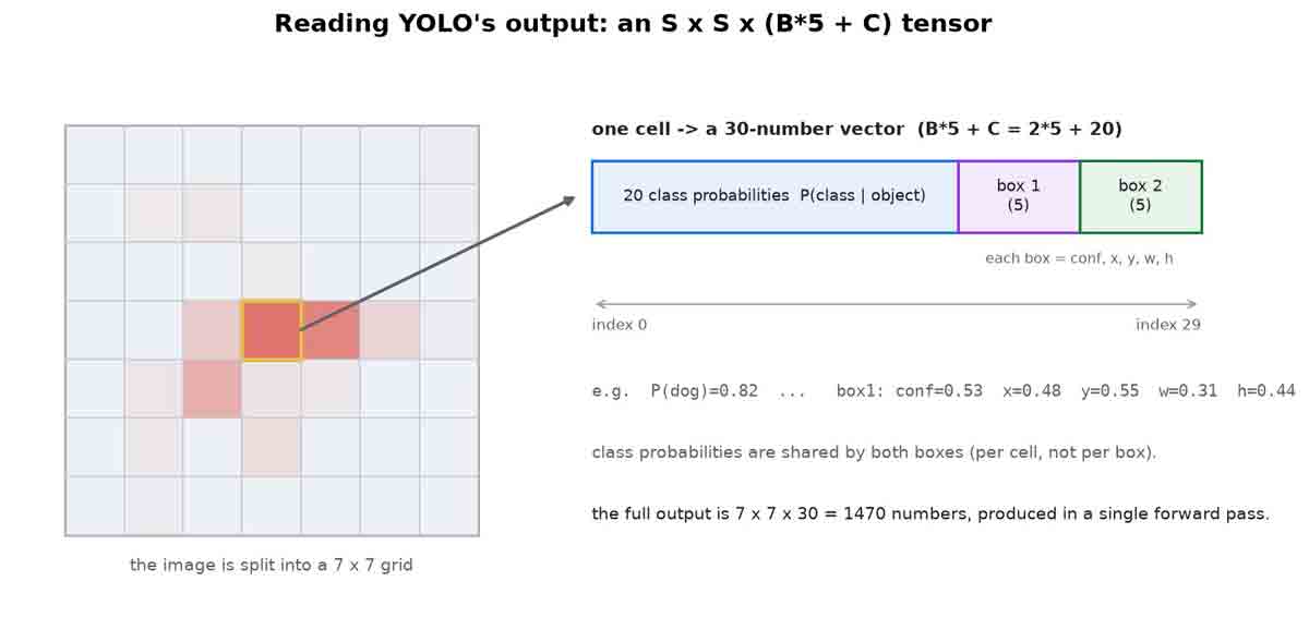
That “shared by both boxes” detail matters: the class probabilities are stored once per cell, not once per box, which is why the vector length is C + B*5 and not B*(5 + C). A cell can therefore describe two boxes but only one class — a real limitation of v1 when two different objects share a cell.

Objects come at every size

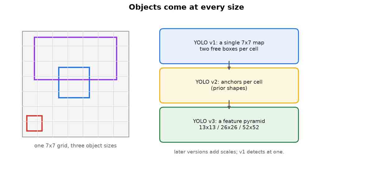
A single 7 × 7 grid handles a mid-sized object comfortably, but it struggles at the extremes: a tiny object may share its cell with others (and the cell only has one class slot), and a very large object spans many cells at once (Fig 6). This is the multi-scale problem, and it is v1's weakest point. Later work answers it with more scales: YOLOv3^[7] predicts on a three-level feature pyramid (13 × 13, 26 × 26, 52 × 52) in the spirit of Feature Pyramid Networks^[8], and SSD^[9] reads boxes off several feature maps of different resolutions. YOLO v1 detects at one scale only — understanding that single grid is the whole point of starting here.

The YOLO label format

To train the network we first turn boxes into the tensor the loss expects. Annotations arrive as pixel corners — xmin, ymin, xmax, ymax — and the YOLO on-disk format normalises each object to one line, class cx cy w h, with every value divided by the image width or height so it lies in [0, 1] (Fig 7). Reading that file is a few lines:

def parse_label_file(path):
    objects = []
    for line in path.read_text().splitlines():
        line = line.strip()
        if not line:
            continue
        # first 5 fields are class + box; VOC labels carry a 6th "difficult" flag
        class_id, x, y, w, h = line.split()[:5]
        objects.append((int(class_id), float(x), float(y), float(w), float(h)))
    return objects

Line 1 defines the parser; lines 3–6 walk the file skipping blank lines; line 8 takes the first five whitespace-separated fields — the class id and the normalised cx, cy, w, h — and tolerates an optional sixth “difficult” flag that VOC adds; line 9 stores each object as a plain tuple; line 10 returns them.

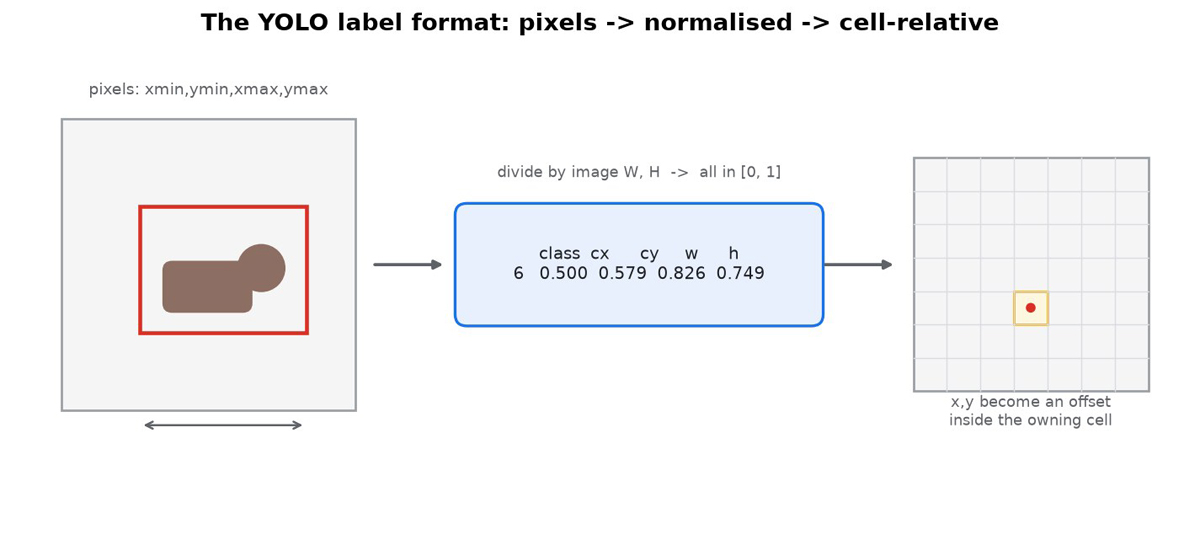
The subtle step is the last one. Encoding places each object into the cell that owns its centre and converts its coordinates into the split convention the network predicts: x and y become an offset relative to that cell (in [0, 1] within the cell), while w and h stay relative to the whole image. The class is written once for the cell, and both box slots are filled so either can become the “responsible” predictor at loss time:

def encode(objects, num_classes, grid_s, num_boxes):
    depth = num_classes + num_boxes * 5
    target = torch.zeros((grid_s, grid_s, depth))
    for class_id, x, y, w, h in objects:
        col = min(int(x * grid_s), grid_s - 1)
        row = min(int(y * grid_s), grid_s - 1)
        if target[row, col, num_classes] == 1.0:
            continue                          # one object per cell: the first wins
        x_cell = x * grid_s - col             # centre offset inside the cell
        y_cell = y * grid_s - row
        target[row, col, class_id] = 1.0      # class is per cell, not per box
        for b in range(num_boxes):
            base = num_classes + b * 5
            target[row, col, base:base + 5] = torch.tensor([1.0, x_cell, y_cell, w, h])
    return target

Lines 2–3 allocate the empty grid_s × grid_s × depth target; lines 5–6 find the cell the centre lands in; lines 7–8 enforce one object per cell, keeping the first when two collide; lines 9–10 convert x, y to the in-cell offset while w, h are left image-relative; line 11 writes the single per-cell class; lines 12–14 fill both box slots with confidence 1 and the same coordinates. Inverting this function recovers the original boxes exactly, which the repository checks with a round-trip test.

One loss to train them all

YOLO's loss is a single sum of squared errors with a few carefully chosen weights (paper section 2.2). Two ideas make it work. First, only one of a cell's two boxes is held responsible for an object — the one whose current prediction has the highest IoU with the ground truth — so the two predictors specialise rather than averaging. Second, the terms are re-weighted: localisation errors are scaled up by λ_coord = 5, and the confidence error for the vast majority of boxes that contain no object is scaled down by λ_noobj = 0.5, so the empty grid does not drown out the few cells that matter.

# each of the B predicted boxes vs the cell's ground-truth box, in image coords
ious = iou_xywh(cell_to_abs(pred_xywh), cell_to_abs(gt_xywh))    # (N,S,S,B)
best_idx = ious.argmax(dim=-1, keepdim=True)                     # the responsible box
resp = torch.zeros_like(ious).scatter_(-1, best_idx, 1.0)
resp = resp * obj.unsqueeze(-1)                 # only in cells that hold an object

# the responsible box's confidence target is its live IoU (Pr(obj) * IoU)
obj_conf_loss = (resp * (pred_conf - ious.detach()) ** 2).sum()
noobj = 1.0 - resp                              # empty cells + the non-responsible box
noobj_conf_loss = LAMBDA_NOOBJ * (noobj * pred_conf ** 2).sum()

Line 2 computes, in image coordinates, the IoU of each of the cell's two predicted boxes against the ground-truth box; line 3 picks the higher one as responsible; lines 4–5 build a mask that is 1 only for that responsible box and only in cells that actually contain an object. Line 8 is the detail most re-implementations get wrong: the confidence target is not a constant 1 but the box's own IoU with the truth (detached so the gradient does not flow back through it), matching the paper's Pr(object) × IoU. Lines 9–10 push every other box — empty cells and the non-responsible box alike — toward zero confidence, down-weighted by λ_noobj. The width and height errors (not shown) are taken on the square roots of w and h, so that a fixed pixel error counts for more on a small box than on a large one.

From tensor to boxes: confidence and non-max suppression

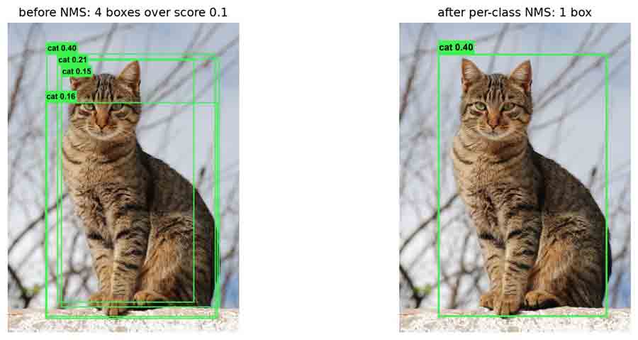
At inference the 7 × 7 × 30 tensor has to become a clean list of detections. Each box's class-specific score is its objectness times the cell's class probability; boxes below a threshold are dropped, and the survivors of each class are thinned by non-max suppression — repeatedly keep the highest-scoring box and discard anything overlapping it too much.

class_probs = pred[..., :C].clamp(0, 1)      # (S,S,C) P(class | object) - already a probability
boxes = pred[..., C:].view(S, S, B, 5)       # (S,S,B,5) the cell's B boxes
conf = boxes[..., 0].clamp(0, 1)             # (S,S,B) objectness, per box
xyxy = cell_to_corners(boxes[..., 1:5])      # cell-relative x,y -> image corners

# a box's score for a class = objectness * class probability (paper's
# "class-specific confidence score")
scores = (conf.unsqueeze(-1) * class_probs.unsqueeze(2)).reshape(-1, C)
xyxy = xyxy.reshape(-1, 4)

detections = []
for class_id in range(C):
    class_scores = scores[:, class_id]
    keep = class_scores >= CONF_THRESHOLD
    cand_boxes, cand_scores = xyxy[keep], class_scores[keep]
    for i in nms(cand_boxes, cand_scores, NMS_IOU):
        detections.append((class_id, cand_scores[i].item(), *cand_boxes[i]))

Lines 1–4 unpack one cell's raw vector: the per-cell class probabilities, its B boxes, each box's objectness, and each box's corners in image coordinates. Line 8 multiplies objectness by class probability to give every box in the grid a class-specific score. Lines 12–16 walk the classes, threshold the scores, and run non-max suppression within each class; line 17 collects the survivors as the final detections. Fig 8 shows why that last step matters.

Line 1 hides a trap worth naming. Those class outputs look like logits, so the reflex is to push them through a softmax — but YOLO's loss regresses them toward a one-hot vector with plain squared error, so a trained cell already emits a probability. Softmax them anyway and a perfect one-hot cell peaks at only e / (e + C − 1): a harmless 0.58 when C = 3, but 0.125 when C = 20, which quietly sits below any sensible confidence threshold and returns almost no detections at all. The loss keeps falling the whole time, because nothing on the training path ever touches the softmax.

Training it, and what it costs

The companion repository trains this network on PASCAL VOC 2007^[11]. Two honest deviations keep it runnable on a single consumer GPU. The paper pretrains a 24-layer DarkNet from scratch on ImageNet^[12]; here an ImageNet-pretrained ResNet-34^[13] trunk feeds the detection head instead — the same 7 × 7 × 30 output, far less compute. The fully-connected head is deliberately kept, because it is exactly what YOLOv2 later discards to switch to anchors. The full loss, grid, and label format are unchanged from the paper. The whole pipeline is built with PyTorch^[14] and torchvision^[15], and the training curve is shown in Fig 9.

The network itself is short to write. A pretrained trunk reduces the image to a feature map, a stride-2 neck lands it on the S × S grid, and a fully-connected head regresses the whole output tensor at once:

class Yolo_V1(nn.Module):
    def __init__(self, num_classes, grid_s, num_boxes):
        super().__init__()
        self.grid_s = grid_s
        self.depth = num_classes + num_boxes * 5      # 20 + 2*5 = 30

        backbone = resnet34(weights=ResNet34_Weights.IMAGENET1K_V1)
        # drop avgpool + fc; at 448x448 the last block emits 512 x 14 x 14
        self.trunk = nn.Sequential(*list(backbone.children())[:-2])

        # neck: 14x14x512 -> 7x7x1024 (the stride-2 conv gets us to the S=7 grid)
        self.neck = nn.Sequential(
            nn.Conv2d(512, 1024, kernel_size=3, stride=2, padding=1),
            nn.BatchNorm2d(1024),
            nn.LeakyReLU(0.1, inplace=True),
            nn.Conv2d(1024, 1024, kernel_size=3, stride=1, padding=1),
            nn.BatchNorm2d(1024),
            nn.LeakyReLU(0.1, inplace=True),
        )

        self.head = nn.Sequential(                    # 7x7x1024 -> 7*7*30
            nn.Flatten(),
            nn.Linear(grid_s * grid_s * 1024, HEAD_HIDDEN),
            nn.LeakyReLU(0.1, inplace=True),
            nn.Dropout(HEAD_DROPOUT),
            nn.Linear(HEAD_HIDDEN, grid_s * grid_s * self.depth),
        )

    def forward(self, x):
        x = self.head(self.neck(self.trunk(x)))
        return x.view(-1, self.grid_s, self.grid_s, self.depth)

Line 5 fixes the per-cell vector at C + B*5 = 30 numbers. Lines 7–9 take a pretrained ResNet-34 and drop its average-pool and classifier, leaving a convolutional stack that turns a 448 × 448 image into a 14 × 14 × 512 feature map. Lines 11–19 are the neck, whose stride-2 convolution halves that map onto the S = 7 grid. Lines 21–27 are the paper's fully-connected head, regressing all 1470 numbers in a single shot — at half the paper's hidden width, which is what lets it train on a 6 GB card. Line 31 folds that flat vector back into the 7 × 7 × 30 tensor: the reshape is the only thing that makes the grid a grid.

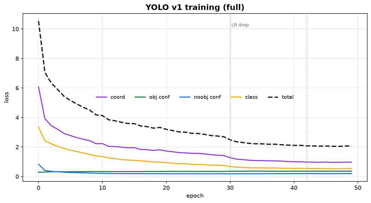
After fifty epochs the detector scores mAP@0.5 = 0.516 across all 4952 VOC 2007 test images. The paper reports 63.4, but trains on VOC 2007 + 2012 together — about three times the images used here. The per-class spread reproduces the weakness the paper names itself: bottle (0.15), pottedplant (0.20) and chair (0.25) sit at the bottom, because a 7 × 7 grid offering two boxes per cell cannot pull apart small, clustered objects, while cat, dog, horse and train all clear 0.70. That gap between the easy classes and the crowded ones is precisely the pressure that produced anchors in YOLOv2.

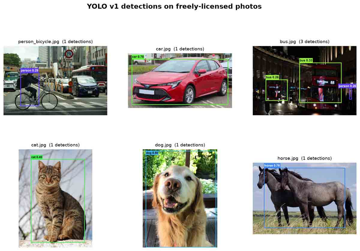
Run on freely-licensed photographs the network has never seen, the trained detector places boxes and labels directly (Fig 10). Every box drawn there survived the same per-class non-max suppression seen earlier in Fig 8.

Key takeaways

• Object detection is classification and box regression done together, for every object at once.
• YOLO replaces the sliding window with a single pass that outputs an S × S × (B*5 + C) tensor — 7 × 7 × 30 for v1.
• Class probabilities are per cell; boxes are per cell too, with x, y stored relative to the cell and w, h relative to the image.
• One box per cell is made “responsible” by IoU; λ_coord and λ_noobj balance localisation against the empty grid.
• v1 has no anchors and one scale; anchors arrive in v2 and multi-scale detection in v3.

The complete, runnable code — the label encoder, the model, the multi-part loss, the decoder with non-max suppression, and the VOC training loop — lives in the companion repository under src/. Full attribution for every photo, dataset, and library is in the repository's RESOURCES.md.

Resources

Every dataset, library, sample photo, and paper cited above — numbered in order of first appearance. Sample photos are used under the licence noted for each; the detection overlays in this article are derivative works of them. Click any bracketed marker such as ^[1] to jump to its entry.

• [1] YOLO v1 — Redmon, Divvala, Girshick, Farhadi, You Only Look Once: Unified, Real-Time Object Detection, CVPR 2016. arXiv:1506.02640
• [2] R-CNN — Girshick, Donahue, Darrell, Malik, Rich Feature Hierarchies for Accurate Object Detection, CVPR 2014. arXiv:1311.2524
• [3] Viola–Jones — Viola, Jones, Rapid Object Detection using a Boosted Cascade of Simple Features, CVPR 2001. IEEE CVPR 2001
• [4] OverFeat — Sermanet et al., Integrated Recognition, Localization and Detection using Convolutional Networks, ICLR 2014. arXiv:1312.6229
• [5] Faster R-CNN — Ren, He, Girshick, Sun, Towards Real-Time Object Detection with Region Proposal Networks, NeurIPS 2015. arXiv:1506.01497
• [6] YOLO9000 / v2 — Redmon, Farhadi, YOLO9000: Better, Faster, Stronger, CVPR 2017. arXiv:1612.08242
• [7] YOLOv3 — Redmon, Farhadi, YOLOv3: An Incremental Improvement, 2018. arXiv:1804.02767
• [8] FPN — Lin et al., Feature Pyramid Networks for Object Detection, CVPR 2017. arXiv:1612.03144
• [9] SSD — Liu et al., SSD: Single Shot MultiBox Detector, ECCV 2016. arXiv:1512.02325
• [10] Cat photo — Alvesgaspar, CC BY-SA 3.0. Wikimedia Commons
• [11] PASCAL VOC — Everingham, Van Gool, Williams, Winn, Zisserman, The PASCAL Visual Object Classes (VOC) Challenge, IJCV 2010. Images for non-commercial research use. host.robots.ox.ac.uk
• [12] ImageNet — Deng et al., ImageNet: A Large-Scale Hierarchical Image Database, CVPR 2009. image-net.org
• [13] ResNet — He, Zhang, Ren, Sun, Deep Residual Learning for Image Recognition, CVPR 2016. arXiv:1512.03385
• [14] PyTorch — Paszke et al., An Imperative Style, High-Performance Deep Learning Library, NeurIPS 2019, BSD-3-Clause. pytorch.org
• [15] torchvision — PyTorch vision models & the pretrained ResNet-34 backbone, BSD-3-Clause. github.com/pytorch/vision
• [16] Cyclist photo — Benlisquare, CC BY-SA 4.0. Wikimedia Commons
• [17] Car photo — Vauxford, CC BY-SA 4.0. Wikimedia Commons
• [18] Bus photo — 0x010C, CC BY-SA 4.0. Wikimedia Commons
• [19] Dog photo — Morphdog, CC BY-SA 4.0. Wikimedia Commons
• [20] Horse photo — François Marchal, CC BY-SA 3.0. Wikimedia Commons