Convolutional Recurrent Neural Network OCR

Reading License Plates End-to-End with a CRNN (CNN + LSTM + CTC)

This project reads the characters off an already-cropped license plate with a single neural network — no per-character segmentation, no hand-tuned thresholds. A convolutional network looks at the plate, a bidirectional LSTM models the character sequence, and a CTC loss aligns the two so the whole strip is transcribed in one shot. It is the sequel to the earlier contour-and-SVM Adhoc_OCR pipeline, and it survives exactly the cases that broke the old one: blur, low resolution, noise, skew, shadows and touching characters.

Code: github.com/babak-abad/CRNN_OCR

Why not the classical adhoc pipeline?

The adhoc project thresholds the plate, finds each character as a separate contour, and classifies each little crop with an SVM. That chain has a single point of failure: segmentation. One smudge, a low-resolution upscale, or two letters that touch, and the character boundaries are wrong — so every downstream classification is wrong too. There is no way for a later stage to recover information the segmentation step already destroyed.

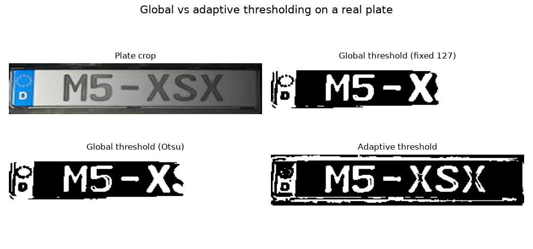
You can see the fragility in the adhoc article's own figures. Thresholding a shadowed plate already loses strokes before a single contour is drawn — a global threshold blacks out half the plate, and even adaptive thresholding leaves the glyphs broken:

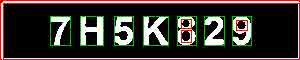
Then every surviving blob has to be split into exactly the right number of contours. Where two characters touch or a screw casts a spot, the split is wrong — here green contours are kept and red ones rejected, and a single bad decision drops or fuses a character for good:

On clean, high-resolution plates the adhoc pipeline is fine. On real roadside photos it is a coin toss. Its own results gallery shows the problem plainly: the reds below are plates whose segmentation failed — blurred, skewed, low-resolution, shadowed and touching-character crops that the contour+SVM chain simply cannot read:

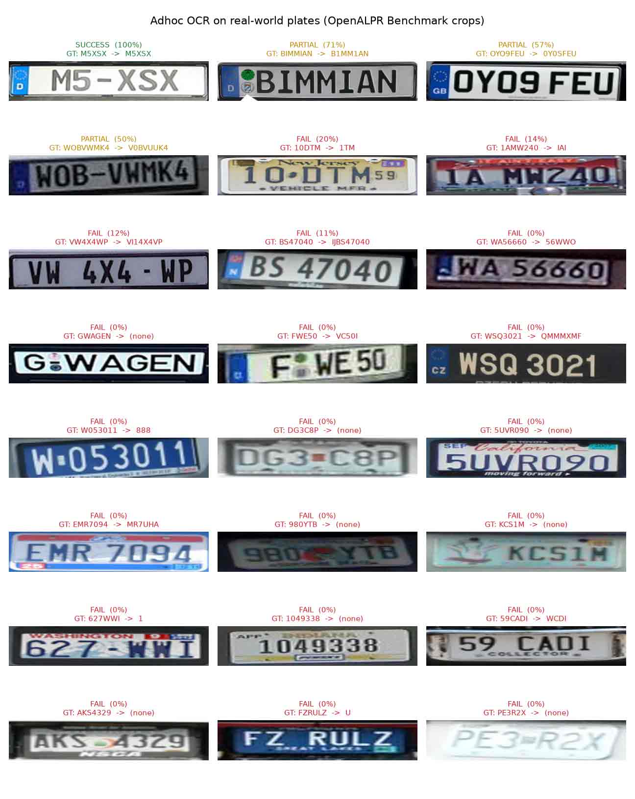
Every one of those red misreads is a plate the CRNN in this project reads without segmenting at all. The CRNN removes segmentation entirely: it slides across the plate from left to right and emits a character sequence, learning from millions of degraded synthetic plates where the boundaries are and how to read through the damage. The result is a model that reads plates the contour pipeline cannot even begin to parse.

Architecture

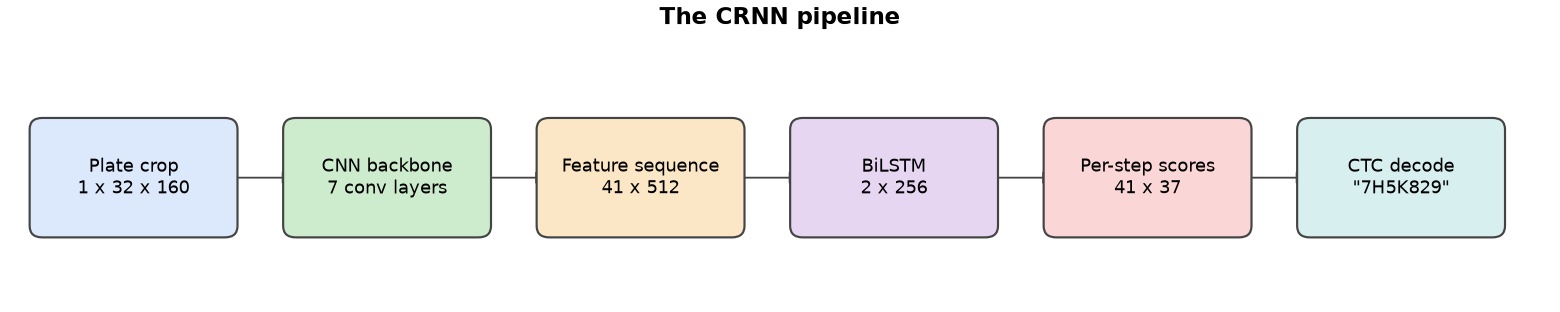
The network has three parts stacked on top of each other:

1. CNN backbone (7 conv layers). It takes a 1×32×160 grayscale crop and progressively collapses the height to a single row while keeping the width high. Two asymmetric pooling steps preserve horizontal resolution so a wide plate still maps to a long enough sequence. Out comes a feature sequence of 41 columns × 512 channels.
2. Bidirectional LSTM (2 layers, 256 units each way). It reads that column sequence left-to-right and right-to-left, so the score for each column is informed by its neighbours on both sides — the context that tells an 8 from a B.
3. CTC head. A linear layer produces, at each of the 41 columns, a score over 37 classes (0-9, A-Z, plus one CTC “blank”). CTC lets the network line up 41 columns with a 5–8 character label without ever being told which column belongs to which character.

Plate crop (1 x 32 x 160)
    -> CNN backbone (7 conv layers)   collapse height, keep width
    -> Feature sequence (41 x 512)
    -> BiLSTM (2 x 256)               read left-to-right and right-to-left
    -> Per-step scores (41 x 37)      36 characters + 1 CTC blank
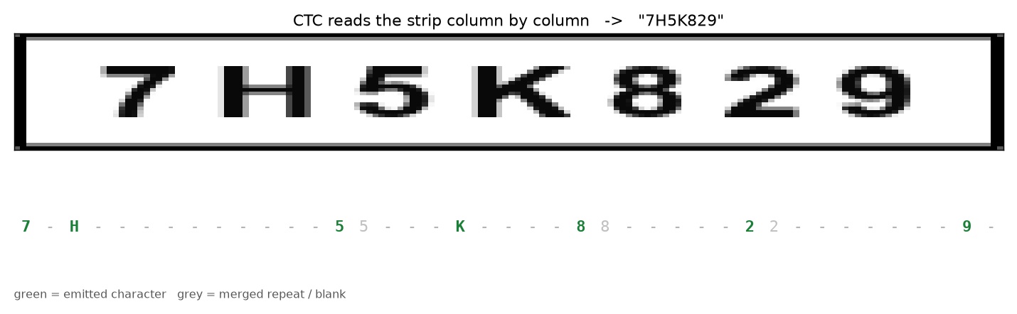
    -> CTC greedy decode              "7H5K829"

How CTC decoding works

CTC is the trick that makes segmentation-free reading possible. The network emits one prediction per column. A single character usually spans several columns, and the gaps between characters emit a special blank symbol (drawn as -). To turn 41 column-predictions into a string, you (1) merge runs of the same repeated label and (2) delete the blanks. So a raw path like 7 7 - H H - 5 5 5 ... collapses to 7H5…. During training, CTC sums over all the column alignments that would collapse to the correct label, so the network is never told where one character ends and the next begins — it discovers that on its own.

A worked example

The reason this is powerful — and the reason it needs no per-character boxes — is that many different column alignments decode to the same text. Take a two-character label AB spread over six columns. All of the paths below are valid; each one merges repeats and drops blanks (-) down to exactly AB:

A A - B B -   ->  AB
- A - - B -   ->  AB
A - - - - B   ->  AB
A A A - B B   ->  AB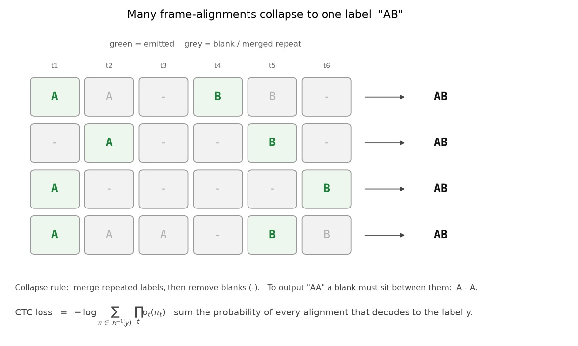

The blank is what makes repeated letters possible: to output AA the path must place a blank between the two A’s (A - A), otherwise the merge step would fuse them into a single A. Training never picks one “correct” alignment. Instead the CTC loss is the negative log of the summed probability of every path that decodes to the label:

loss(y) = -log ∑π ∈ ℋ-1(y) ∏t pt(πt)

where ℋ is the collapse operation and ℋ^-1(y) is the set of all column paths that collapse to the target y. That sum over exponentially many paths is computed efficiently with a forward–backward dynamic program (the same idea as in HMMs), so a single backward pass nudges the network toward all plausible alignments at once. The network discovers where characters begin and end entirely on its own.

What the network sees

Every crop is converted to a 32×160 grayscale image and normalised before it enters the CNN:

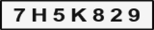
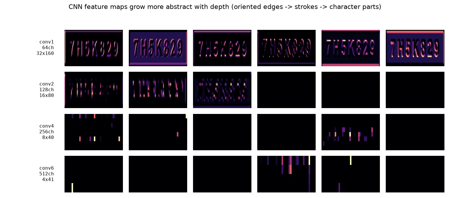
The convolutional backbone turns that image into feature maps, and they grow more abstract with depth. The montage below taps four points in the stack. The first layer (conv1, 64 channels at full 32×160) reacts to oriented edges and strokes — some maps fire on vertical strokes, some on the character tops, some on the plate border. Deeper layers (conv2, conv4, conv6) fire on larger, sparser character parts while the spatial grid shrinks — by conv6 the height is almost collapsed to the single row that becomes the feature sequence handed to the LSTM:

Training data is generated, not downloaded

A CRNN needs a lot of labelled plates. Instead of collecting and hand-labelling them, the project renders random 0-9 / A-Z strings with real system fonts and then degrades each one on the fly with the same distortions a roadside camera introduces: rotation, perspective, motion and Gaussian blur, aggressive downscaling, sensor noise, JPEG artefacts, uneven lighting, and negative letter-spacing so glyphs touch. Because the label is simply the string that was drawn, no annotated dataset is required to train. Training is a CTC loss on these synthetic plates, Adam with a OneCycle schedule; roughly 4000 iterations at batch 64 takes about five minutes on an RTX 3060.

Real plate crops are still useful for evaluation. Genuine photos from the public OpenALPR Benchmark — each plate cropped from the supplied annotation and labelled with its ground-truth text — let you measure accuracy on real images or fine-tune.

Reading the code, file by file

The whole project is small — a handful of short files. Below is each one with the lines that matter, walked through in order. The layout is:

src/config.py      every knob in one place (image size, alphabet, model width, training)
src/charset.py     text <-> class indices, and CTC greedy decoding
src/plate_gen.py   render a clean plate crop from a text string
src/dataset.py     degrade rendered plates and serve them as tensors
src/model.py       the CRNN itself: CNN backbone + BiLSTM + CTC head
src/train.py       the training loop (CTC loss, validation, checkpointing)
src/recognize.py   load a trained model and read a crop
run_pipeline.py    command-line entry point to read one plate

1. src/config.py — one place for every number

Everything the rest of the code reads — image geometry, the alphabet, layer widths, training length — lives here, so there is a single source of truth and no magic numbers scattered around:

IMG_HEIGHT = 32
IMG_WIDTH  = 160

CHARSET = "0123456789ABCDEFGHIJKLMNOPQRSTUVWXYZ"
BLANK = 0
NUM_CLASSES = len(CHARSET) + 1        # 36 characters + 1 blank = 37

CNN_OUT    = 512                      # channels leaving the CNN backbone
RNN_HIDDEN = 256                      # hidden units per LSTM direction
RNN_LAYERS = 2

MIN_PLATE_LEN = 5
MAX_PLATE_LEN = 8

BATCH_SIZE    = 64
LEARNING_RATE = 1e-3
ITERATIONS    = 5000

In lines 1–2 the input geometry is fixed: every crop becomes a 32×160 grayscale image before it reaches the network, tall enough to keep glyph detail and wide enough to give CTC room to work. Line 4 defines the CHARSET — the 36 characters the model can output. Line 5 reserves index 0 as the CTC blank, and line 6 makes NUM_CLASSES = 37 (36 real characters plus that blank); this single + 1 is what ties the alphabet to the CTC head. Lines 8–10 size the network: 512 channels out of the CNN, a 256-unit LSTM in each direction, 2 layers deep. Lines 12–13 say generated plates are 5 to 8 characters long, and lines 15–17 set the training regime — batch 64, learning rate 1e-3, 5000 iterations by default. Changing any of these numbers changes the whole project consistently, because every other file imports config instead of hard-coding.

2. src/charset.py — text to indices, and CTC decoding

The network works in class indices, not letters, so this file translates both ways and also performs the CTC “collapse” that turns 41 raw column-predictions into a readable string:

_char_to_idx = {ch: i + 1 for i, ch in enumerate(CHARSET)}
_idx_to_char = {i + 1: ch for i, ch in enumerate(CHARSET)}

def encode(text):
    return [_char_to_idx[ch] for ch in text.upper() if ch in _char_to_idx]

def decode_greedy(indices):
    text = []
    prev = -1
    for idx in indices:
        idx = int(idx)
        if idx != prev and idx != BLANK:
            text.append(_idx_to_char.get(idx, ""))
        prev = idx
    return "".join(text)

Lines 1–2 build the two lookup tables. Note the i + 1: character "0" is class 1, not 0, because class 0 is permanently the blank. Method encode (lines 4–5) upper-cases the label and maps each known character to its index, silently dropping anything outside the alphabet — that is what turns "7H5K829" into a list of target indices for the loss.

Method decode_greedy (lines 7–15) is the CTC best-path decoder, and it is exactly the two-rule collapse described earlier. Line 9 seeds prev to -1 so the first real character is always emitted. The test on line 12 is the whole trick: a character is kept only when it differs from the previous column (that merges runs of repeats) and is not the blank (that drops the gaps). So a raw path like 7 7 - H H - 5 emits 7, skips the repeat, skips the blank, emits H, skips its repeat and blank, emits 5 — giving 7H5. Line 14 remembers the current index for the next iteration's comparison, and line 15 joins the kept characters into the final string.

3. src/plate_gen.py — drawing a clean plate

There is no downloaded dataset; the training images are drawn. This file renders one clean plate crop from a text string using a real system font. The same renderer feeds both the demo plates and the raw canvas that dataset.py later degrades:

def render_plate(text, font_path=None, colors=None, spacing=None, border=True,
                 native_height=64, rng=random):
    font_path = font_path if font_path is not None else rng.choice(FONTS)
    bg, fg = colors if colors is not None else rng.choice(COLOR_SCHEMES)
    if spacing is None:
        spacing = rng.randint(2, 10)

    font_size = int(native_height * 0.62)
    font = ImageFont.truetype(str(font_path), font_size) if font_path else ImageFont.load_default()

    boxes  = [font.getbbox(ch) for ch in text]
    widths = [max(1, b[2] - b[0]) for b in boxes]
    text_w = sum(widths) + spacing * (len(text) - 1)
    ...
    x = (width - text_w) // 2
    for ch, w, (l, t, r, b) in zip(text, widths, boxes):
        y = (height - (b - t)) // 2 - t
        draw.text((x - l, y), ch, fill=tuple(fg[::-1]), font=font)
        x += w + spacing
    ...
    if border:
        edge = tuple(int(0.55 * c) for c in fg)
        cv2.rectangle(bgr, (1, 1), (width - 2, height - 2), edge, max(1, height // 32))
    return bgr

Lines 3–4 pick a random font and a random colour scheme (white-on-black, yellow UK rear, blue EU, and so on) unless the caller pins them, so no two generated plates look identical. The key parameter is spacing on lines 5–6: it is the gap in pixels between glyphs, and it is allowed to be negative. A negative spacing makes the letters touch or overlap — deliberately manufacturing the joined-character case that defeats contour segmentation but not the CRNN.

Lines 11–13 measure each glyph's bounding box so the whole string can be centred. The loop on lines 16–19 draws each character in turn, advancing x by the glyph width plus the (possibly negative) spacing, so overlapping glyphs are laid down on top of each other exactly the way a low-quality plate stamp would. Lines 21–23 stroke a darker border around the plate, and line 24 returns the finished BGR image. Nothing here is labelled by hand — the label is the text argument.

4. src/dataset.py — degrading plates into training data

This is where a clean render becomes a realistic, hard training image. First a library of individual degradations, each one modelling something a real camera does. Here are three representative ones:

def _downscale(img, factor):
    h, w = img.shape[:2]
    small = cv2.resize(img, (max(4, int(w / factor)), max(4, int(h / factor))),
                       interpolation=cv2.INTER_AREA)
    return cv2.resize(small, (w, h), interpolation=cv2.INTER_LINEAR)

def _noise(img, sigma, rng):
    out = img.astype(np.float32) + rng.np.randn(*img.shape) * sigma
    return np.clip(out, 0, 255).astype(np.uint8)

def _brightness_gradient(img, strength, rng):
    h, w = img.shape[:2]
    gx, gy = rng.r.uniform(-1, 1), rng.r.uniform(-1, 1)
    grad = gx * np.linspace(-1, 1, w)[None, :] + gy * np.linspace(-1, 1, h)[:, None]
    grad = grad / (np.abs(grad).max() + 1e-6)
    factor = (1.0 + strength * grad)[..., None]
    return np.clip(img.astype(np.float32) * factor, 0, 255).astype(np.uint8)

Method _downscale (lines 1–5) is the low-resolution simulator: it shrinks the plate by factor and then blows it back up to full size, so fine detail is genuinely destroyed — exactly the upscaling artefact that ruins contour segmentation. Method _noise (lines 7–9) adds Gaussian sensor noise of standard deviation sigma and clips back into [0, 255]. Method _brightness_gradient (lines 11–17) builds a linear light ramp in a random direction (lines 13–14), normalises it (line 15) and multiplies the image by it (lines 16–17), producing the uneven shadow or glare a plate has under a streetlight. The file has more of these — rotation, perspective, Gaussian and motion blur, JPEG compression, and even random screw-head specks.

The images arrive as tensors through one small converter:

def to_tensor(img_bgr):
    gray = cv2.cvtColor(img_bgr, cv2.COLOR_BGR2GRAY)
    gray = cv2.resize(gray, (config.IMG_WIDTH, config.IMG_HEIGHT), interpolation=cv2.INTER_AREA)
    x = (gray.astype(np.float32) / 255.0 - 0.5) / 0.5
    return torch.from_numpy(x).unsqueeze(0)          # (1, H, W)

Method to_tensor is the single door into the network. Line 2 drops colour — a plate reader does not need it. Line 3 forces the fixed 160×32 geometry from config. Line 4 normalises pixels from [0, 255] to roughly [-1, 1], which keeps the CNN's activations well-scaled. Line 5 adds the single channel dimension so the shape is (1, H, W). Everything — training, evaluation, inference — passes through this function, so the network always sees data the same way.

The random augmentation pipeline chains those degradations, each applied with its own probability so every sample is unique:

def augment_train(img, rng):
    if rng.r.random() < 0.6:
        img = _rotate(img, rng.r.uniform(-8, 8))
    if rng.r.random() < 0.4:
        img = _perspective(img, 0.10, rng)
    if rng.r.random() < 0.4:
        img = _brightness_gradient(img, rng.r.uniform(0.2, 0.6), rng)
    if rng.r.random() < 0.5:
        if rng.r.random() < 0.5:
            img = _gaussian_blur(img, rng.r.randint(1, 3) * 2 + 1)
        else:
            img = _motion_blur(img, rng.r.randint(3, 9), rng)
    if rng.r.random() < 0.5:
        img = _downscale(img, rng.r.uniform(1.5, 4.0))
    if rng.r.random() < 0.5:
        img = _noise(img, rng.r.uniform(4, 20), rng)
    if rng.r.random() < 0.25:
        img = _screws(img, rng)
    if rng.r.random() < 0.5:
        img = _jpeg(img, rng.r.randint(25, 75))
    return img

Each if in augment_train rolls a die and, perhaps, applies one degradation, so a single clean render can come out rotated and blurred and down-scaled and noisy. Lines 2–3 rotate by up to ±8°; lines 4–5 apply a perspective warp; lines 6–7 add a shadow gradient; lines 8–12 pick either Gaussian or motion blur; lines 13–14 crush the resolution; lines 15–16 add noise; lines 17–18 stamp screw specks; lines 19–20 add JPEG artefacts. Because these compose, the network sees effectively unlimited variety and learns to read through the damage rather than memorising clean glyphs.

Finally the torch Dataset generates one fresh sample per index:

class SyntheticPlates(Dataset):
    def __getitem__(self, idx):
        rng = _Rng(self.seed * 1_000_003 + idx)
        text = plate_gen.random_text(rng=rng.r)
        spacing = rng.r.randint(-6, 1) if (self.train and rng.r.random() < 0.15) else None
        img = plate_gen.render_plate(text, spacing=spacing, rng=rng.r)
        img = augment_train(img, rng) if self.train else augment_eval(img, rng)
        target = torch.tensor(charset.encode(text), dtype=torch.long)
        return to_tensor(img), target, text

def collate(batch):
    imgs, targets, texts = zip(*batch)
    images = torch.stack(imgs, 0)
    target_lengths = torch.tensor([len(t) for t in targets], dtype=torch.long)
    targets_cat = torch.cat(targets) if len(targets) else torch.zeros(0, dtype=torch.long)
    return images, targets_cat, target_lengths, list(texts)

Method __getitem__ (lines 2–9) builds a sample on demand. Line 3 seeds a fresh random generator from the index, so the same index always yields the same plate — the dataset is infinite yet perfectly reproducible. Line 4 chooses a random string, line 5 gives a 15% chance of the joined-character (negative-spacing) case during training, line 6 renders it, and line 7 degrades it. Line 8 turns the label text into target indices with charset.encode, and line 9 returns the image tensor, the target, and the original text.

Method collate (lines 11–16) packs a batch the way nn.CTCLoss wants it. Because plates have different lengths, the targets are concatenated into one flat tensor (line 15) with a separate list of lengths (line 14), rather than padded into a rectangle. The images, being a fixed size, stack normally (line 13).

5. src/model.py — the CRNN itself

This is the heart of the project. The constructor builds the CNN backbone as one nn.Sequential, then the LSTM and the linear head:

self.cnn = nn.Sequential(
    *_conv_block(1, 64),
    nn.MaxPool2d(2, 2),                                   # 32x160 -> 16x80
    *_conv_block(64, 128),
    nn.MaxPool2d(2, 2),                                   # -> 8x40
    *_conv_block(128, 256, batch_norm=True),
    *_conv_block(256, 256),
    nn.MaxPool2d((2, 2), (2, 1), (0, 1)),                 # -> 4x41
    *_conv_block(256, 512, batch_norm=True),
    *_conv_block(512, 512),
    nn.MaxPool2d((2, 2), (2, 1), (0, 1)),                 # -> 2x42
    nn.Conv2d(512, config.CNN_OUT, kernel_size=2, stride=1, padding=0),
    nn.BatchNorm2d(config.CNN_OUT),
    nn.ReLU(inplace=True),                                # -> 1x41
)
self.rnn = nn.LSTM(config.CNN_OUT, rnn_hidden, num_layers=rnn_layers,
                   bidirectional=True, dropout=0.2 if rnn_layers > 1 else 0.0)
self.fc = nn.Linear(rnn_hidden * 2, num_classes)

Read the comments down the right edge and you can watch the tensor shrink. The input is 32×160. The first two pools (lines 3 and 5) are ordinary 2×2, halving both dimensions to 8×40. The two pools on lines 8 and 11 are the crucial ones: their stride is (2, 1) — 2 vertically, 1 horizontally — so they keep halving the height while barely touching the width. That asymmetry is what preserves horizontal resolution so a wide plate still becomes a long sequence. By line 14 the height has collapsed to 1 and the width is 41: the 41-column feature sequence. Line 16 defines the bidirectional 2-layer LSTM over those 512-channel columns, and line 18's linear head maps its 2×256 output to the 37 class scores per column.

def forward(self, x):
    feat = self.cnn(x)                    # (B, C, 1, W')
    b, c, h, w = feat.size()
    assert h == 1, f"CNN height must collapse to 1, got {h}"
    feat = feat.squeeze(2)                # (B, C, W')
    feat = feat.permute(2, 0, 1)          # (W', B, C) = (T, B, C)
    seq, _ = self.rnn(feat)               # (T, B, 2*hidden)
    return self.fc(seq)                   # (T, B, num_classes) raw logits

Method forward is short because the shapes do the work. Line 2 runs the backbone. Line 4 asserts the height really did collapse to 1 — a guard that catches any accidental geometry change. Line 5 drops that height dimension, and line 6 is the pivotal reshape: it permutes the axes to (W', B, C), i.e. (time, batch, channels), which is exactly the layout an LSTM expects — the image width has literally become the time axis of a sequence. Line 7 runs the BiLSTM and line 8 returns raw per-column logits, ready to hand straight to nn.CTCLoss or to greedy decoding.

6. src/train.py — the training loop

Training is a standard supervised loop with CTC as the loss. The setup:

criterion = nn.CTCLoss(blank=config.BLANK, zero_infinity=True)
optimizer = torch.optim.Adam(model.parameters(), lr=lr)
scheduler = torch.optim.lr_scheduler.OneCycleLR(optimizer, max_lr=lr, total_steps=iterations)

Line 1 creates the CTC loss, telling it that class BLANK = 0 is the blank; zero_infinity=True guards against the infinite losses CTC can produce when a target is longer than the sequence. Line 2 is Adam, and line 3 is the OneCycle schedule that warms the learning rate up and then anneals it — the reason ~4000 iterations is enough to reach high accuracy.

logits = model(images)                                 # (T, B, C)
input_lengths = torch.full((images.size(0),), logits.size(0), dtype=torch.long)
loss = criterion(logits.log_softmax(2), targets, input_lengths, target_lengths)

optimizer.zero_grad()
loss.backward()
nn.utils.clip_grad_norm_(model.parameters(), 5.0)
optimizer.step()
scheduler.step()

This is the per-step core. Line 1 runs the model to get the (T, B, C) logits. Line 2 tells CTC how long each input sequence is — here every input is the full T = 41 columns. Line 3 computes the loss: note log_softmax over the class axis, which is what nn.CTCLoss expects, together with the concatenated targets and their target_lengths from collate. Lines 5–8 are the usual zero-grad / backward / step, with line 7 clipping the gradient norm to 5.0 to keep the recurrent part stable, and line 9 advances the OneCycle schedule.

if step % config.VAL_EVERY == 0 or step == iterations:
    seq_acc, char_acc = evaluate(model, val_loader, device)
    if seq_acc >= best:
        best = seq_acc
        save(model, seq_acc, char_acc)

Every VAL_EVERY steps the model is evaluated on a held-out split (line 2), and it is written to disk only when it improves (lines 3–5), so the saved crnn_ocr.pt is always the best model seen, not merely the last. Method evaluate reports two numbers: sequence accuracy (the whole plate correct) and character accuracy (fraction of characters correct), both decoded with the same decode_greedy from charset.py.

7. src/recognize.py — reading a crop

Inference loads the checkpoint and runs one image through:

@torch.no_grad()
def recognize(image_bgr, model, device):
    tensor = dataset.to_tensor(image_bgr).unsqueeze(0).to(device)   # (1, 1, H, W)
    probs = model(tensor).softmax(2)[:, 0, :]                       # (T, C)
    path = probs.argmax(1).tolist()
    gray = cv2.resize(cv2.cvtColor(image_bgr, cv2.COLOR_BGR2GRAY),
                      (config.IMG_WIDTH, config.IMG_HEIGHT))
    return Recognition(text=charset.decode_greedy(path),
                       confidence=_path_confidence(probs, path), gray=gray)

Line 1's @torch.no_grad() disables gradient tracking for speed. Line 3 reuses the exact same to_tensor the training data went through — training and inference must preprocess identically or accuracy collapses. Line 4 turns logits into probabilities and drops the batch axis to give a (T, C) table: for each of the 41 columns, a probability over the 37 classes. Line 5 takes the arg-max at each column — the greedy path — and line 8 collapses it to text with decode_greedy. Method _path_confidence (line 9) averages the probability at just the columns that actually emitted a character, giving the confidence number printed with the result.

8. run_pipeline.py — the command-line entry point

A thin wrapper so you can read a plate from the shell:

image = cv2.imread(args.image)
model, device = recognize.load_model(args.model)
rec = recognize.recognize(image, model, device)
print(f"Recognized text : {rec.text}")
print(f"Confidence      : {rec.confidence:.2f}")
cv2.imwrite(out, recognize.annotate(image, rec))

Line 1 reads the crop, line 2 loads the trained model, and line 3 runs the recognition just described. Lines 4–5 print the decoded string and its confidence, and line 6 writes an annotated JPG — the upscaled plate with the prediction printed underneath — via recognize.annotate.

CRNN vs. the classical pipeline, easy to hard

The comparison below runs both readers over the same eight plates, ordered from a clean render to a combined-degradation nightmare. The green/amber/red labels show exact match, mostly-right, and failure.

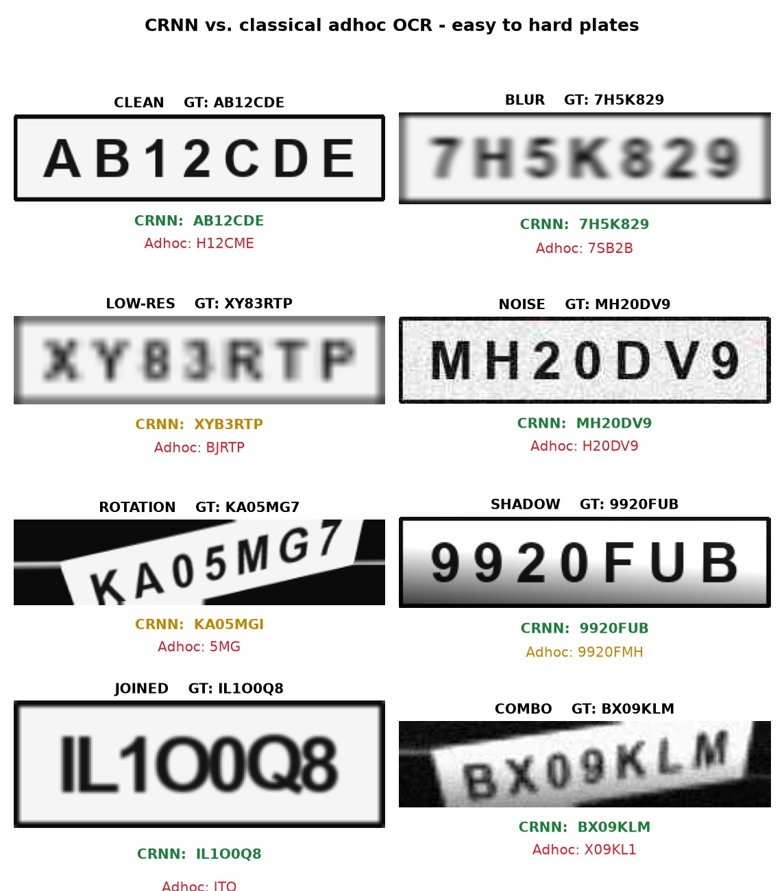
On this run the CRNN read 6 of 8 plates exactly (and got most characters right on the other two), while the contour-and-SVM adhoc pipeline read 0 of 8 exactly — its segmentation dropped or split characters on every degraded plate. That gap is the whole point: the adhoc pipeline fails the moment a character boundary is ambiguous, and the CRNN never needs the boundary in the first place. The same blurred, low-resolution, shadowed and touching-character plates that show up as red failures in the adhoc gallery above are read correctly here.

More plates: a larger synthetic batch

Eight plates could be luck, so here are twelve more — fresh strings, a different random seed, and the same spread of degradations (blur, low resolution, noise, skew, shadow, and touching characters). Both readers see exactly the same crops.

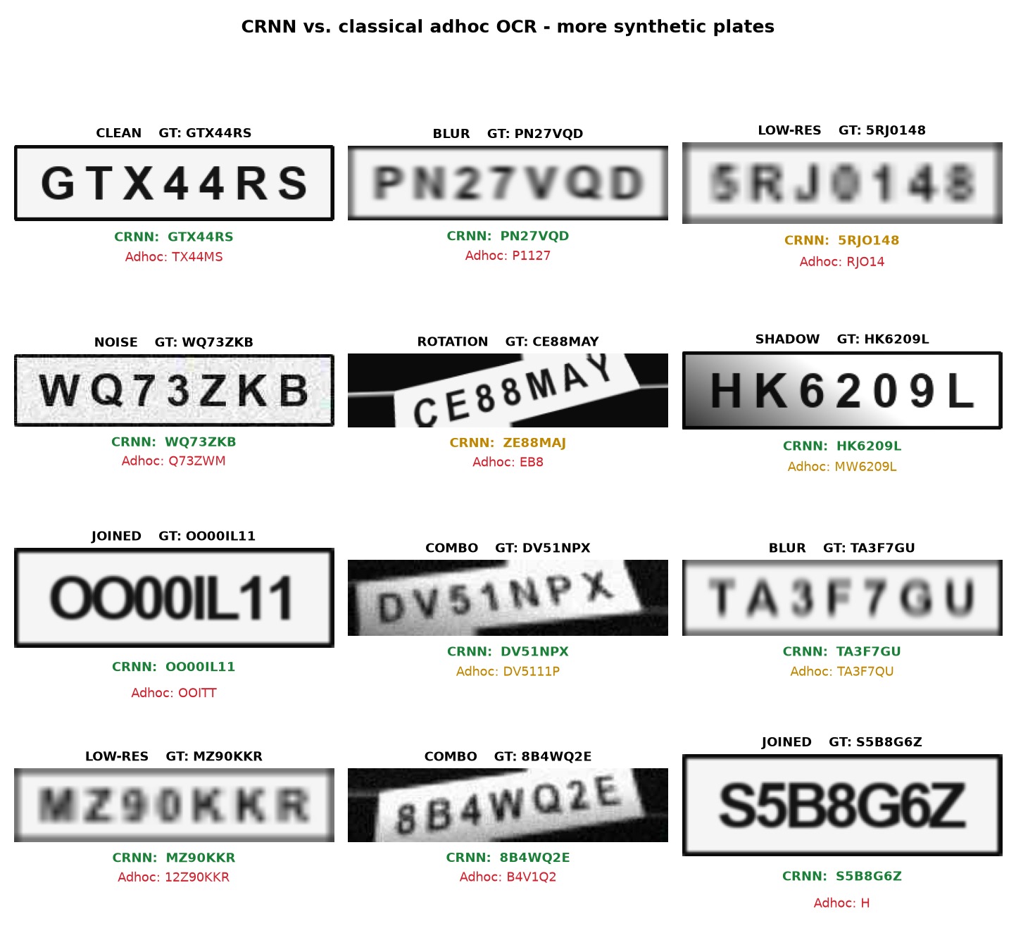
On this batch the CRNN read 10 of 12 plates exactly (≈96% of individual characters correct), missing only a rotated CE88MAY and taking the confusable O/0 in 5RJ0148. The adhoc pipeline read 0 of 12 exactly (≈27% of characters) — its segmentation dropped a leading glyph, fused touching pairs, or split a noisy stroke into two on every single plate. The pattern is the same as before: the moment a character boundary is ambiguous, the classical pipeline is lost, while the CRNN never needs the boundary.

Real-world plates, straight off the benchmark

Synthetic plates are the training distribution, so the honest test is genuine roadside photos. The crops below come from the public OpenALPR Benchmark — real US and EU plates with state banners, slogans, mounting frames, embossed characters and low contrast, cropped straight from the annotation and fed to both readers unchanged. This CRNN has never seen a real plate (it was trained purely on generated images), so real photos are out of its training distribution; the six shown here are the crops where that synthetic training still carries over, and they make the contrast with the classical pipeline clearest.

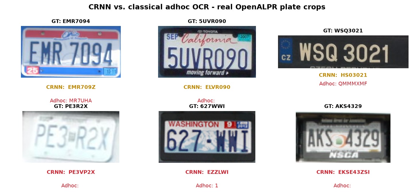
Be clear about what this shows: these are the model's best real crops, not a full benchmark. Even here it is not perfect — it has never seen a real plate — but it reads through the state banners and embossing to recover about half the characters (EMR7094 → EMR709Z, off by a single glyph; 5UVR090 → ELVR090; WSQ3021 → HS03021), whereas the contour+SVM pipeline returns a stray character or nothing at all. On plenty of other real crops neither reader is usable off the shelf; closing that gap is exactly what fine-tuning on a real ALPR dataset does (see the Limitations below). The architecture is already reading through the degradations, it simply needs a few real plates to calibrate to real fonts and backings.

Results

Trained purely on generated plates:

Quantity	Value
Classes	37 (0-9, A-Z, + CTC blank)
Input	32 × 160 grayscale
Parameters	~8.7 M
Held-out sequence accuracy (medium-difficulty synthetic)	~99%
Held-out character accuracy	~99.8%

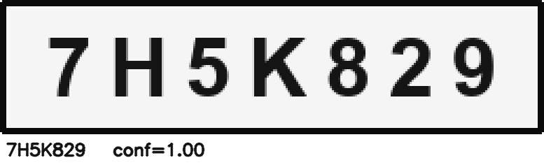
A single clean crop reads with full confidence:

Running it yourself

# 1. TRAIN the network (CTC loss on generated plates) -> models/crnn_ocr.pt
python -m src.train --iterations 4000

# 2. READ one plate crop
python run_pipeline.py --image data/samples/plate_7H5K829.jpg

Limitations

The model is trained on Latin 0-9 / A-Z plates only; it does not read Persian, Arabic or Chinese scripts without retraining on that alphabet. It also expects an already-cropped plate — a real deployment still needs a separate detector to find and crop the plate first. Accuracy on genuine photos improves further by fine-tuning on a real ALPR dataset such as RodoSol-ALPR or the OpenALPR Benchmark.

Full code and instructions: github.com/babak-abad/CRNN_OCR