Neural Networks Taxonomy

In little more than a decade, neural networks have moved from an academic curiosity to the engine behind image search, machine translation, protein-structure prediction, and the conversational assistants millions now use every day. Yet there is no single “neural network” behind all of this — there is a sprawling family tree of architectures, dozens of distinct families, each invented to fix a problem the previous generation could not solve. This article walks that tree from the ground up: what a neural network is, and then, family by family, where each design came from, what it is good at, and where it falls short.

What is a neural network?

A neural network is a function built by stacking many small, simple units into layers. Each unit takes a set of numbers, multiplies them by learned weights, adds the results, and passes the sum through a non-linear activation such as ReLU or tanh. Stacked deep enough and trained on enough examples, that arrangement can approximate astonishingly complex relationships — from pixels to object labels, from audio to text. The network in Fig 1 shows the smallest interesting example: an input layer, one hidden layer, and an output layer, every unit in one layer connected to every unit in the next.

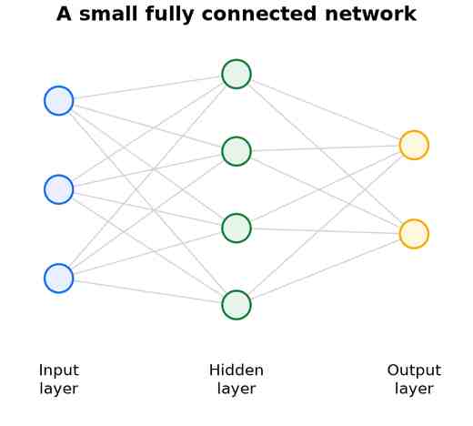
Learning means adjusting those weights so the network's output moves closer to the desired answer. The workhorse algorithm is backpropagation: it measures the error at the output and pushes it backwards through the layers, telling each weight how to change. Almost every architecture in this article — however exotic — is trained by some form of this idea, and the whole field is often called deep learning once the layers grow numerous.^[1]

From brains to artificial neurons

The metaphor is old. In 1943, McCulloch and Pitts proposed that a biological neuron — which gathers signals through its dendrites, sums them in the cell body, and fires down its axon when the total crosses a threshold — could be modelled as a simple logical unit.^[2] The artificial neuron keeps exactly that shape, as Fig 2 makes explicit: inputs scaled by weights stand in for dendrites, the weighted sum plays the role of the soma, and the activation function is the firing decision. The analogy is loose — real neurons are far richer — but it gave the field its name and its first designs.

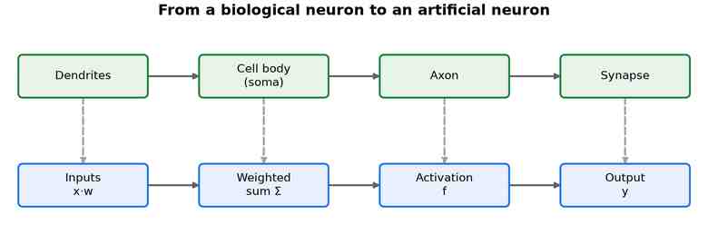
What distinguishes modern networks from this early model is not just depth but the differentiability of every component. The choice of activation function, for instance, dictates how gradients flow; ReLU (Rectified Linear Unit) passes positive values unchanged and zeros out negatives, which avoids the saturation that plagued earlier sigmoid-based networks. This seemingly minor change, popularised around 2010, was one of the unsung enablers of the deep-learning revolution, because it kept error signals alive across dozens of layers.

Their role in modern systems

What changed between the 1943 metaphor and today's systems is scale. Three ingredients arrived together: large labelled datasets, graphics processors fast enough to train big models, and a set of architectural ideas — convolution, gating, attention — that let networks exploit the structure of images, sequences, and graphs. Together they turned neural networks into the default tool for perception and generation, displacing hand-engineered features across vision, speech, and language.^[1]

What they are good at — and where they struggle

Neural networks excel whenever the mapping from input to output is complex, noisy, and backed by plenty of examples but hard to write down as rules: recognising a cat, transcribing speech, translating a sentence. Their weaknesses are the mirror image. They are data-hungry and compute-hungry; they can be confidently wrong on inputs unlike anything they were trained on; and their reasoning is opaque, which matters in medicine, law, and finance. Much of the family tree that follows is a history of trading one of these weaknesses away — usually at the cost of adding structure that suits a particular kind of data.

The rest of this article is organised as a tour of that tree. Each of the following pages takes one family of architectures: what it is, when and why it was introduced, a diagram of its characteristic shape, what it is used for, and where it stumbles. Where one family was invented to cure another's disease, the text links the two.

1. Feedforward Neural Networks (FNN)

The feedforward neural network is the family the introduction already described: units arranged in layers, information flowing strictly forward from input to output, with no loops. Its most common form is the multilayer perceptron (MLP), a stack of fully connected Dense layers each followed by a non-linearity, sketched in Fig 3. Everything else in this taxonomy can be read as an MLP with extra structure bolted on to suit a particular kind of data.

Origins and rise

The lineage starts with Rosenblatt's perceptron in 1958, a single trainable layer that could separate linearly separable classes.^[3] Its inability to solve even the XOR problem stalled the field until the 1986 popularisation of backpropagation by Rumelhart, Hinton, and Williams made it practical to train the hidden layers of a multilayer network.^[4] Soon after, the universal approximation theorem showed that a feedforward network with a single sufficiently wide hidden layer can approximate any continuous function to arbitrary accuracy^[5] — a reassuring result that says nothing about how to learn such a network efficiently, which is exactly what the specialised families that follow address.

1.1 Fully connected (dense)

Beyond the plain MLP, the fully connected branch holds several notable variants. The deep autoencoder stacks an encoder and a mirror-image decoder to squeeze data into a low-dimensional code and reconstruct it; Hinton and Salakhutdinov showed such a network could beat classical PCA at dimensionality reduction once its layers were pre-trained greedily.^[6] That same layer-by-layer pre-training defined the deep belief network (DBN), a stack of restricted Boltzmann machines that briefly made very deep networks trainable before ReLU activations and better initialisation made the ritual unnecessary.^[7] A different branch trades learning for speed: the extreme learning machine (ELM) fixes the hidden weights at random and solves only the output layer in closed form,^[8] an idea echoed by the random vector functional link (RVFL) network and the broad learning system (BLS), which widen the network rather than deepen it.

1.2 Partially and locally connected

Connecting every unit to every other is wasteful when the input has local structure. A locally connected layer keeps the spatial grid of an image but gives each position its own unshared weights — the halfway house between a dense layer and the weight-sharing convolution of the next family. The pioneering example was Fukushima's neocognitron (1980), a hierarchy of local feature detectors and pooling cells that fed directly into the design of convolutional networks.^[9]

1.3 Linear and shallow models

At the shallow end sit the single-layer models that started the field. Rosenblatt's perceptron and Widrow and Hoff's ADALINE (1960) are linear classifiers trained by simple weight updates; MADALINE wired several ADALINEs together into one of the first practical multi-layer trainers. Logistic regression is the same object seen from statistics — a one-layer network with a sigmoid output. All share the perceptron's ceiling: with no hidden layer they can only draw linear boundaries, the very wall that backpropagation was popularised to break.

Applications

• Tabular prediction: credit scoring, churn, and risk models over fixed-length feature vectors.
• The final classification or regression “head” on top of almost every other architecture in this article.
• Function approximation inside larger systems — value estimates in reinforcement learning, for example.

Strengths and limitations

Strengths	Limitations
Universal approximators; simple and fast to train.	Ignore spatial or temporal structure in the input.
A natural output head for any model.	Fully connected layers scale badly to raw images or long sequences.
Work well on fixed-length feature vectors.	Prone to overfitting without heavy regularisation.

That second limitation — blindness to structure — is precisely what the next family fixes. Feeding a million-pixel image into a dense layer needs an impossible number of weights; convolutional networks share weights across the image to make vision tractable.

2. Convolutional Neural Networks (CNN)

A convolutional neural network replaces full connectivity with a small learnable filter that slides across the image, reusing the same weights at every position. That single idea — weight sharing plus local receptive fields — slashes the parameter count and builds in translation invariance: a feature detector that finds an edge in one corner finds it everywhere. A typical CNN alternates conv layers with pool layers that shrink the spatial size, then finishes with a feedforward head, as in Fig 4. Mathematically, a 2D convolution computes a dot product between the filter and a local patch of the input at every location: (I * K)(i,j) = sum_m sum_n I(i+m, j+n) K(m,n). The translational equivariance of this operation is the reason a CNN can recognise a face regardless of where it appears in the frame.

Origins and rise

LeCun's LeNet-5 read handwritten digits for the postal service in the 1990s,^[10] but the family exploded in 2012 when AlexNet won the ILSVRC competition on the ImageNet dataset by a wide margin, using ReLU activations and two GPUs to train a then-enormous model.^[11][12] VGG then showed that stacking many small 3×3 filters worked better than a few large ones,^[13] but pushing depth further ran into the vanishing-gradient problem: error signals faded before they reached the early layers. ResNet solved it in 2015 with the residual connection — the dashed skip in Fig 4 — which adds a layer's input to its output so gradients have a short path back, making networks hundreds of layers deep trainable at last.^[14]

2.1 Image-classification backbones

The backbone zoo is the convolutional network's heartland. After AlexNet and VGG, GoogLeNet's Inception module ran filters of several sizes in parallel to widen a network cheaply,^[15] and ResNet's skip connection unlocked real depth. DenseNet took connectivity to its limit, feeding every layer's output to all later layers,^[16] while ResNeXt and Wide ResNet tuned the width-versus-depth trade-off. A parallel push shrank backbones to fit a phone: MobileNet swapped full convolutions for cheap depthwise-separable ones,^[17] and ShuffleNet, SqueezeNet, and GhostNet squeezed out more. EfficientNet balanced depth, width, and resolution with one compound scaling rule,^[18] a line that runs up through RegNet and RepVGG to ConvNeXt, which modernised a plain ResNet with Transformer-era training tricks to rival the vision transformers it was answering.^[19] The search for optimal backbones also spurred the Neural Architecture Search methods; EfficientNet's scaling rule, for instance, emerged from a systematic grid search over depth, width, and resolution, proving that balancing these three dimensions is far more effective than scaling any one in isolation.

2.2 Object detection

Detection adds where to what. The two-stage lineage — R-CNN, Fast R-CNN, and Faster R-CNN, which folded region proposals into the network itself^[20] — trades speed for accuracy, and Cascade and Sparse R-CNN refined it. One-stage detectors instead predict boxes directly for real-time speed: the YOLO family (v1 through v10, plus YOLOX and PP-YOLO),^[21] SSD, and RetinaNet, whose focal loss fixed the foreground-background imbalance that had capped one-stage accuracy.^[22] Anchor-free designs (FCOS, CenterNet, CornerNet) dropped the hand-tuned anchor boxes, and DETR recast detection as direct set prediction with a Transformer, removing non-maximum suppression from the pipeline^[23] — a bridge to the Transformer family.

2.3 Segmentation

Segmentation labels every pixel. The fully convolutional network (FCN) made this practical by turning the classification head into a dense one;^[24] U-Net's symmetric encoder-decoder with skip connections became the default for medical and scientific imaging,^[25] and the DeepLab series added atrous (dilated) convolutions and multi-scale pooling for scene parsing.^[26] Instance segmentation, which separates individual objects, is led by Mask R-CNN, which bolts a mask branch onto Faster R-CNN,^[27] alongside YOLACT and SOLO. Panoptic methods (Panoptic FPN, Mask2Former, OneFormer) unify the two, and the Segment Anything Model (SAM) turned segmentation into a promptable foundation task trained on a billion masks.^[28]

2.4 Video and 3D CNNs

Extending the convolution to time gives video models. C3D and I3D inflate 2D filters into 3D to learn motion, the latter bootstrapping from image-pretrained weights and the Kinetics dataset.^[29] R(2+1)D factorises space and time for efficiency, X3D scales a tiny network along several axes, and SlowFast runs two pathways — a slow one for appearance and a fast one for motion — that fuse for strong action recognition.^[30]

2.5 Restoration and super-resolution

The same machinery reconstructs images. SRCNN first showed a three-layer network could upscale images better than hand-crafted interpolation;^[31] EDSR and RCAN deepened it, and adversarial training brought photo-realistic texture — SRGAN and then ESRGAN, whose enhanced generator set the quality bar.^[32] Real-ESRGAN pushed it to real-world degradations, and Transformer-based restorers such as SwinIR and HAT now lead the field.^[33]

Applications

• Image classification, object detection, and semantic segmentation.
• Medical imaging, satellite and industrial inspection, and photo restoration.
• A feature extractor inside larger multimodal and generative systems.

Strengths and limitations

Strengths	Limitations
Parameter-efficient through weight sharing.	Local filters see only a small region at a time.
Built-in translation invariance.	Weaker at modelling long-range, global relationships.
Mature, fast, and hardware-friendly.	Fixed grid assumes image-like input.

The limitation that a convolution only sees a local patch is one the Transformer later removed for vision, letting every location attend to every other. Lighter fixes also exist: attention modules reweight a convolutional network's own features, and architecture search can design the backbone automatically. For data that arrives as a sequence rather than a grid, though, the field first turned to a different design entirely.

3. Recurrent Neural Networks (RNN)

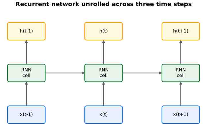
A recurrent neural network processes a sequence one step at a time, keeping a hidden state that carries information forward from earlier steps. The same cell is applied at every step, so the network can handle sequences of any length; drawn “unrolled” in time it looks like Fig 5, with the hidden state passed sideways from one step to the next. This makes the RNN a natural fit for text, audio, and time series. The recurrence can be written as h_t = f(h_{t-1}, x_t), where the same function f and the same weight matrix are reused at every timestep. This weight-tying makes the model compact and, in principle, capable of capturing dependencies of arbitrary length.

Origins and rise

Elman's simple recurrent network in 1990 established the pattern,^[34] but plain RNNs suffered the same vanishing-gradient problem as deep feedforward stacks: they forgot information from more than a few steps back. The breakthrough was the long short-term memory (LSTM) cell of Hochreiter and Schmidhuber in 1997, which added a protected memory cell and multiplicative gates that decide what to keep, forget, and output.^[35] The gates are computed as sigmoid functions of the current input and previous hidden state, producing values between 0 and 1 that act as soft switches. The cell state passes information almost unchanged across long time spans, which is why LSTMs can retain context over hundreds of steps. The lighter gated recurrent unit (GRU) of 2014 achieved much the same with fewer gates.^[36] Through the mid-2010s, gated RNNs powered machine translation, speech recognition, and the first strong language models.

3.1 Simple recurrent networks

The earliest designs simply feed the previous state back as an extra input. Elman's network loops the hidden layer; Jordan's loops the output layer. Both are trained by backpropagation through time (BPTT), which unrolls the loop into a deep feedforward graph and applies ordinary backpropagation. Their habit of forgetting anything more than a few steps back is exactly what the gated cells below were built to cure.

3.2 LSTM and its variants

The LSTM's protected cell spawned a family of tweaks. Peephole connections let the gates read the cell state directly; the bidirectional LSTM runs one pass forward and one backward so every step sees future as well as past context;^[37] and stacked and grid LSTMs add depth across layers and dimensions. ConvLSTM swaps the cell's matrix multiplies for convolutions, letting it model spatiotemporal data such as radar maps and video.^[38]

3.3 GRU and its variants

The GRU merged the LSTM's forget and input gates into a single update gate. Lighter still are the minimal gated unit, which keeps just one gate, and Light GRU; ConvGRU applies the same convolutional trick as ConvLSTM. In practice GRU and LSTM trade blows, with the GRU often preferred for its smaller state and faster training.

3.4 Efficient recurrent networks

A recurrent cell's step-to-step dependency blocks the parallelism GPUs thrive on, and several designs claw it back. The quasi-recurrent neural network (QRNN) interleaves convolutions with a minimal recurrent pooling step;^[39] the simple recurrent unit (SRU) drops the state-to-state matrix so most of the work runs in parallel;^[40] and the independently recurrent neural network (IndRNN) makes the neurons within a layer independent, enabling very deep, long-memory recurrence.^[41] FastGRNN and Delta RNN target tiny, on-device budgets.

3.5 Memory-augmented networks

Some tasks need an addressable memory far larger than a hidden state. The neural Turing machine (NTM) couples a recurrent controller to an external memory it reads and writes through differentiable attention;^[42] its successor, the differentiable neural computer (DNC), added dynamic memory allocation and could answer graph and reasoning questions.^[43] End-to-end memory networks stack several soft-attention lookups over a stored set of facts — a direct ancestor of the attention that would soon eclipse recurrence entirely.^[44]

3.6 Reservoir computing

Reservoir computing takes the opposite tack: leave the recurrent weights fixed and random, and train only a linear readout on top. The echo state network does this with a rate-based reservoir,^[45] while the liquid state machine uses a pool of spiking neurons;^[46] next-generation reservoir computing reproduces the effect with an explicit polynomial feature map. Cheap to train, these models shine at chaotic time-series prediction.

Applications

• Speech recognition and text-to-speech.
• Time-series forecasting and anomaly detection.
• Streaming and on-device tasks where inputs arrive one step at a time.

Strengths and limitations

Strengths	Limitations
Handle variable-length sequences naturally.	Sequential processing cannot be parallelised across time.
Compact state, well suited to streaming.	Still struggle with very long-range dependencies.
Gated cells tame the vanishing gradient.	Slow to train on long sequences.

That first limitation — the step-by-step bottleneck that stops an RNN from using modern hardware fully — is what the Transformer was designed to eliminate, and its removal reshaped the entire field.

4. Transformer Networks

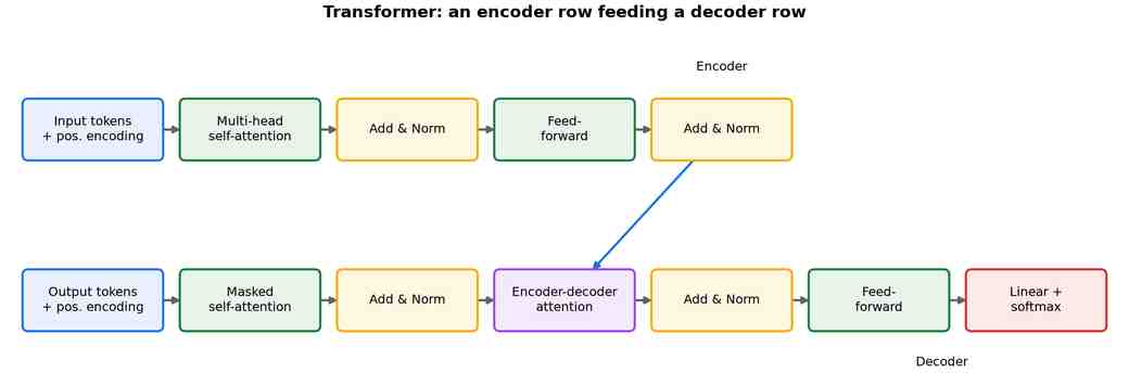
The Transformer replaces recurrence with self-attention: every element of a sequence looks directly at every other element and decides how much each one matters. Because those comparisons happen all at once rather than step by step, the whole sequence is processed in parallel — the exact bottleneck that slowed recurrent networks down. The architecture stacks multi-head attention and feedforward blocks into an encoder and a decoder, wired together as in Fig 6. At its core, the attention mechanism computes a weighted sum of values based on the similarity between queries and keys: Attention(Q,K,V) = softmax(QK^T / sqrt(d_k)) V. The scaling factor sqrt(d_k) prevents dot-products from growing too large and pushing the softmax into saturation, which stabilises gradients. The multi-head formulation runs this computation several times in parallel, with different learned projections, allowing the model to attend to different aspects of the input simultaneously.

Origins and rise

The design was introduced in 2017 in the paper “Attention Is All You Need,” which showed that attention alone, with no recurrence or convolution, set a new state of the art in machine translation while training far faster.^[47] Two directions followed almost immediately. BERT used only the encoder, pre-trained to fill in masked words, and became the backbone of search and classification.^[48] The GPT line used only the decoder to predict the next token, and scaling it to hundreds of billions of parameters produced the general-purpose language models behind today's assistants.^[49] Attention then crossed into vision: the Vision Transformer (ViT) cut an image into patches and treated them as a sequence, matching or beating convolutional networks given enough data.^[50]

4.1 The base architecture

The original 2017 design is an encoder–decoder built from two repeated pieces: multi-head self-attention and a position-wise feed-forward network, each wrapped in a residual connection and layer normalisation.^[47] Attention itself is a scaled dot-product: every token emits a query, a key, and a value, and each output is a weighted average of values whose weights come from query–key similarity. Running several heads in parallel lets one layer attend to different relationships at once. Because attention is order-blind, the input is tagged with positional encodings so the network can still tell first token from last. Almost every model below keeps this skeleton and changes only which half it uses, how attention is computed, or what the network is trained on.

4.2 Natural-language models

Keeping only the encoder gives a bidirectional model that reads a whole passage at once, suited to understanding rather than generation. BERT set the template, pre-training on masked-word prediction before fine-tuning for search, classification, and question answering.^[48] RoBERTa showed the recipe was under-trained and won large gains from more data and longer schedules alone;^[51] ELECTRA swapped masked-word filling for a more sample-efficient “spot the replaced token” objective;^[52] and DeBERTa's disentangled attention, which encodes content and position separately, pushed the family past human baselines on several benchmarks.^[53] ALBERT, DistilBERT, and Megatron-BERT trade accuracy against size and speed.

Keeping only the decoder gives an autoregressive model that predicts the next token, and this is the branch that became today's large language models. Scaling GPT to hundreds of billions of parameters revealed that a single next-token objective, given enough data, yields few-shot learning on tasks it was never explicitly trained on.^[49] The Chinchilla study then reset the field's scaling laws, showing that most large models were badly under-trained and that data and parameters should grow together.^[54] Google's PaLM scaled the idea to 540 billion parameters,^[55] while Meta's LLaMA proved that far smaller, carefully trained open models could rival them,^[56] seeding an open ecosystem of Mistral, Falcon, and Gemma — and the mixture-of-experts Mixtral, which sparsely routes each token to a few expert sub-networks to grow capacity without a matching rise in compute.^[57]

Keeping both halves suits sequence-to-sequence tasks such as translation and summarisation. T5 cast every language problem as text-to-text, so one model and one objective could translate, summarise, and answer questions.^[58] BART pre-trained by corrupting text and learning to reconstruct it, excelling at generation and summarisation;^[59] multilingual and instruction-tuned variants — mT5, Flan-T5, mBART, Pegasus, and ProphetNet — extend the same encoder–decoder core.

4.3 Vision transformers

Attention reached images by slicing a picture into fixed-size patches and feeding them as a sequence — the Vision Transformer, which matched convolutional networks once given enough data.^[50] DeiT removed the giant-dataset requirement with distillation and stronger augmentation, training a competitive ViT on ImageNet alone.^[60] Swin Transformer reintroduced a convolution-like hierarchy, computing attention within shifted local windows so cost grows linearly with image size, which made transformers practical backbones for detection and segmentation.^[61] A parallel thread pursued self-supervised pre-training: BEiT predicted masked visual tokens in the style of BERT,^[62] the masked autoencoder (MAE) reconstructed heavily masked pixels and made large-scale pre-training cheap,^[63] and DINO showed that self-distillation makes ViT features segment objects with no labels at all, later scaled up as DINOv2.^[64] PVT, CvT, Twins, PoolFormer, CaiT, CrossViT, and iBOT fill in the design space between these poles.

4.4 Efficient and long-context transformers

Self-attention's cost grows with the square of sequence length, so a whole subfamily attacks that quadratic wall. Sparse-attention models let each token see only a subset of the others: Longformer combines a sliding window with a few global tokens,^[65] and BigBird adds random links while proving it retains the full model's expressive power.^[66] Reformer groups similar tokens with locality-sensitive hashing,^[67] while Linformer and Performer approximate attention with low-rank or kernel-based maps that make it linear.^[68] A different tack keeps attention exact but rewrites its implementation: FlashAttention reorders the computation to minimise reads and writes to GPU memory, giving large speed-ups and far longer contexts with identical results.^[69]

4.6 Decision and generalist transformers

The same sequence model can drive action as well as language. The Decision Transformer reframes reinforcement learning as sequence modelling: conditioned on a desired return, it simply predicts the next action, sidestepping explicit value functions and bootstrapping.^[70] Gato pushed the generalist idea furthest, training one transformer to caption images, hold a conversation, stack blocks with a robot arm, and play Atari from a single set of weights.^[71] Both point toward the multimodal systems of family 15, where a shared transformer backbone fuses text, images, audio, and action.

Applications

• Large language models, translation, summarisation, and code generation.
• Vision, speech, and multimodal models that mix text with images or audio.
• Protein and molecule modelling, and increasingly reinforcement learning and robotics.

Strengths and limitations

Strengths	Limitations
Model long-range relationships directly.	Attention cost grows with the square of sequence length.
Highly parallel; scale to enormous datasets.	Very data- and compute-hungry to train well.
One architecture spans text, vision, and audio.	Little built-in prior, so small-data regimes suffer.

5. Generative Models

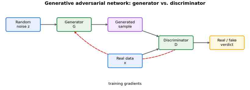
The families so far mostly discriminate — they map an input to a label. A generative model instead learns the distribution of the data well enough to sample new examples from it: fresh images, audio, or text that never existed. Several distinct designs share this goal. The generative adversarial network (GAN) in Fig 7 pits two networks against each other; the variational autoencoder (VAE) and diffusion models take other routes to the same end. The common thread is that they all learn a parametric approximation of the true data distribution, usually by minimising a divergence such as the Kullback–Leibler divergence or the Wasserstein distance, and once trained, they can generate new samples by drawing from a simple prior (e.g., a standard Gaussian) and passing it through the learned generator.

Origins and rise

Goodfellow's GAN in 2014 framed generation as a game between a generator and a discriminator, and for several years produced the sharpest synthetic images available.^[72] In parallel, the VAE gave a probabilistic, more stable route to a smooth latent space.^[73] The current wave belongs to diffusion models, introduced as DDPM in 2020, which learn to reverse a gradual noising process and generate by denoising pure noise.^[74] Moving that process into a compressed latent space produced Stable Diffusion and the text-to-image systems now in wide use.^[75] Notably, these generators are not a rival branch of the tree so much as a way of using it: their building blocks are convolutional and Transformer networks turned toward synthesis.

5.1 Generative adversarial networks

The GAN casts generation as a game: a generator turns noise into samples while a discriminator learns to tell them from real data.^[72] DCGAN pinned down the convolutional recipe that first made this train reliably,^[76] but the objective was notoriously unstable and prone to mode collapse. The Wasserstein GAN reframed the loss around a smoother distance and largely tamed that instability,^[77] while self-attention (SAGAN) let the generator model long-range structure across a whole image.^[78]

Scale and architecture then chased photorealism. Progressive growing built images coarse-to-fine for the first convincing megapixel faces,^[79] StyleGAN's style-based generator gave separate control over coarse and fine attributes and set the bar for face synthesis,^[80] and BigGAN scaled class-conditional generation to ImageNet.^[81] A second thread mapped one image domain to another: Pix2Pix learned paired translation such as sketch-to-photo,^[82] and CycleGAN removed the need for paired data with a cycle-consistency loss.^[83] GANs also drove super-resolution — SRGAN and ESRGAN^[32] — and audio synthesis (WaveGAN, HiFi-GAN), while text-to-image GANs such as StackGAN and AttnGAN were later overtaken by diffusion.

5.2 Variational autoencoders

The VAE takes a probabilistic route: an encoder maps each input to a distribution in a latent space, and a decoder reconstructs from samples of it, trained to keep that space smooth and continuous.^[73] Constraining the latent code — as in β-VAE — encourages disentangled, individually meaningful factors. The most influential branch made the code discrete: VQ-VAE quantises it against a learned codebook, sidestepping blurry reconstructions and pairing naturally with autoregressive or Transformer priors,^[84] a design extended by VQ-VAE-2 and NVAE. VQGAN added an adversarial loss on top, and its perceptual latent codes became the compression stage that makes latent diffusion practical.^[85]

5.3 Autoregressive models

An autoregressive model factorises data into an ordered product and predicts one element at a time, each conditioned on all before it. For images, PixelRNN and PixelCNN generate pixel by pixel,^[86] a line that led to ImageGPT and to the VQ-VAE-plus-Transformer stack behind the first DALL·E. For audio, WaveNet generates raw waveforms sample by sample and reset the bar for speech synthesis,^[87] with WaveRNN and SampleRNN trading quality for speed. The approach gives exact likelihoods and stable training, at the cost of slow sequential sampling.

5.4 Diffusion models

Diffusion models, today's dominant image generators, learn to reverse a gradual noising process: corrupt an image with many small steps of Gaussian noise, then train a network to undo each step so that sampling can start from pure noise.^[74] DDIM made sampling far faster by turning the reverse process deterministic and skipping steps,^[88] while the score-based SDE view unified diffusion with score matching and continuous-time dynamics.^[89] The turning point for adoption was the finding that a well-tuned diffusion model beats GANs on image quality.^[90]

Moving the process into a VAE's compressed latent space gave latent diffusion — Stable Diffusion — cutting cost enough for consumer hardware,^[75] with SDXL scaling it to higher resolution and quality.^[91] Cascaded pixel-space systems such as Imagen and DALL·E 2/3 took a parallel path (their text-to-image side belongs to the multimodal family). Because sampling is the bottleneck, fast solvers such as DPM-Solver and consistency models cut the step count from thousands to a handful.^[92] The same denoising recipe now drives video (Make-A-Video), 3D (DreamFusion), and speech (DiffWave).

5.5 Flow-based models

A normalising flow builds a generator from a stack of exactly invertible transformations, so it can both sample and compute exact likelihoods — unlike a GAN or VAE. RealNVP introduced the coupling layers that keep the Jacobian tractable,^[93] and Glow added invertible 1×1 convolutions for high-quality image synthesis.^[94] NICE, Flow++, and FFJORD extend the idea, and rectified flow — which learns straight-line transport between noise and data — has re-emerged at the heart of recent systems such as Stable Diffusion 3.

5.6 Energy-based models

An energy-based model learns a scalar energy that is low on real data and high elsewhere, then samples by descending that landscape — the oldest generative idea here. The restricted Boltzmann machine and the deep belief networks stacked from it were central to the deep-learning revival of the mid-2000s.^[7] Modern revivals such as JEM show that an ordinary classifier is secretly an energy-based model and can be trained to generate as well as classify.^[95] Sampling remains the hard part, which is why the families above, with their direct sampling paths, now dominate.

Applications

• Text-to-image and image editing, super-resolution, and inpainting.
• Speech and music synthesis.
• Data augmentation and simulation where real examples are scarce.

Strengths and limitations

Strengths	Limitations
Produce novel, high-fidelity samples.	GAN training can be unstable and mode-collapse.
Diffusion is stable and covers the data well.	Diffusion sampling is slow, needing many steps.
Learn reusable latent representations.	Raise real concerns over misuse and training-data rights.

6. Graph Neural Networks (GNN)

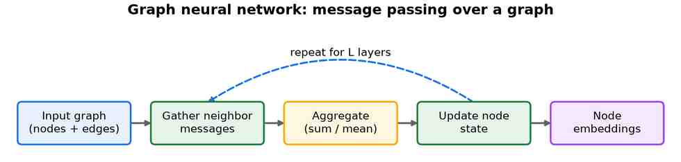
A graph neural network works on data shaped as a graph — nodes joined by edges — rather than a grid or a sequence. It runs on message passing: each node repeatedly gathers information from its neighbours, aggregates it, and updates its own state, as in Fig 8. In effect it generalises the weight sharing of a convolutional network from a regular pixel grid to arbitrary, irregular connectivity. The aggregation function is typically a permutation-invariant operation (sum, mean, or max) to respect the fact that neighbours have no intrinsic order, and the update step is often an MLP that combines the node's own representation with the aggregated message.

Origins and rise

Early work defined convolution in the graph's spectral domain, but the field took off with the simple, scalable graph convolutional network (GCN) of Kipf and Welling in 2017.^[96] Graph Attention Networks (GAT) then let each node weigh its neighbours by learned importance — the same idea as the attention modules and Transformer that appear elsewhere in this tree.^[97]

Spectral methods

The earliest graph networks borrowed from signal processing, defining convolution through the graph's Laplacian spectrum. ChebNet approximated those spectral filters with Chebyshev polynomials, making them local and cheap to compute,^[98] and the GCN simplified this to a single-hop averaging rule that became the field's default baseline.^[96] Purely spectral filters are tied to one fixed graph, however, which pushed the field toward the spatial view below.

Spatial message passing

Spatial methods define a layer directly as message passing over neighbours, and most modern GNNs are variants of it. GraphSAGE made the scheme inductive by sampling and aggregating a fixed number of neighbours, so a trained model generalises to unseen nodes and enormous graphs.^[99] The message-passing neural network framework then unified many of these designs under one gather-and-update template.^[100] GAT weighs neighbours by learned attention,^[97] while the graph isomorphism network (GIN) was built to be as discriminative as the Weisfeiler–Lehman test, clarifying exactly how expressive message passing can be.^[101] GATv2, PNA, GatedGCN, and EdgeConv (DGCNN) extend the aggregation and edge-handling machinery.

Geometric and higher-order networks

Because plain message passing cannot tell some structures apart, one line adds higher-order information — SubGNN, k-GNNs, and graph substructure networks (GSN) count subgraphs or reason over node tuples. A closely related thread targets molecules and 3D point sets, where geometry matters: SchNet uses continuous-filter convolutions to model atomic interactions,^[102] DimeNet and GemNet add directional and angular detail, and SE(3)-Transformers build in rotation and translation equivariance so predictions respect physical symmetry.^[103] Equiformer and TorchMD-Net carry the same idea into molecular dynamics.

Spatiotemporal graphs

When a graph also evolves in time — traffic sensors, moving skeletons, sensor arrays — spatiotemporal GNNs combine graph convolution across space with sequence modelling across time. ST-GCN applies this to skeleton-based action recognition,^[104] while DCRNN and Graph WaveNet forecast traffic by pairing diffusion or dilated-convolution dynamics with a learned graph structure.^[105] MTGNN extends the approach to general multivariate time series.

Graph transformers

As Transformers spread, researchers asked whether attention over all nodes could replace message passing. Graphormer showed it can, encoding graph structure through carefully designed positional and edge biases to win molecular-property benchmarks.^[106] GraphGPS offers a modular recipe that mixes local message passing with global attention, and TokenGT, SAT, and Grit explore other ways to feed graph structure to a Transformer.

Self-supervised graph learning

Labels on graphs are often scarce, so contrastive and bootstrapping methods pre-train on structure alone. GraphCL learns representations invariant to graph augmentations such as edge dropping and subgraph sampling,^[107] JOAO automates the choice of those augmentations, and BGRL drops the need for negative samples by bootstrapping, scaling self-supervision to very large graphs.

Applications

• Molecular property prediction and drug discovery.
• Recommendation, fraud detection, and social-network analysis.
• Traffic forecasting and physical simulation on meshes.

Strengths and limitations

Strengths	Limitations
Handle arbitrary relational structure.	Deep stacks over-smooth, blurring nodes together.
Invariant to node ordering.	Hard to scale to graphs with billions of edges.
Reuse one operator across the whole graph.	Sensitive to how the graph itself was built.

7. Self-Organizing Maps (SOM) & Competitive Learning

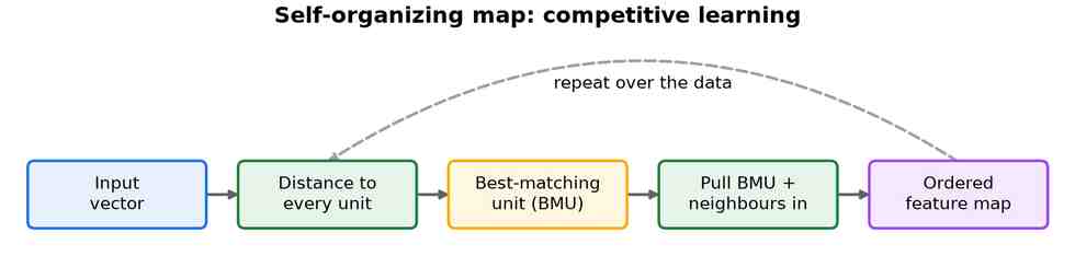
A self-organizing map is an unsupervised network that projects high-dimensional data onto a low-dimensional grid while preserving its topology: similar inputs end up near each other on the map. It learns by competition rather than backpropagation — for each input the closest unit “wins” and is nudged, along with its neighbours, toward that input, as Fig 9 shows. This makes it a very different animal from the backprop-trained feedforward networks that dominate the rest of this tree. The neighbourhood radius is typically annealed over training, starting large to form a global ordering and shrinking to refine local details.

Origins and rise

Kohonen introduced the map in 1982, and it became a staple of exploratory data analysis and visualisation through the 1990s.^[108] Related competitive schemes — learning vector quantization, neural gas, growing networks — share the winner-take-all idea. For modern representation learning the family has largely been overtaken by the self-supervised metric-learning methods discussed later.

The Kohonen map and its variants

Kohonen's original map fixes a rectangular or hexagonal grid of units and adapts them to the data.^[108] Because computing every winner online is slow, the batch SOM updates all units together in one sweep, and hierarchical variants stack maps for coarse-to-fine structure. The growing hierarchical SOM (GHSOM) removes the need to fix the grid in advance, expanding both the size of each map and the depth of the hierarchy to match the data's complexity.^[109]

Growing and topology-learning networks

A related family drops the fixed grid entirely and lets the network's own graph grow to fit the data. Neural gas sorts all units by their distance to each input and adapts them in that order, learning a topology without any predefined layout.^[110] Growing neural gas (GNG) and its utility-driven GNG-U variant add and delete units and edges on the fly, while growing when required (GWR) inserts a new unit whenever the existing ones fit an input poorly, which suits non-stationary data.^[111] The topology-representing network formalises the edges these methods learn as an induced Delaunay graph.

Learning vector quantization

Where the maps above are unsupervised, learning vector quantization (LVQ) is their supervised cousin: it places labelled prototypes in the input space and, for each training example, pulls the nearest correct prototype closer and pushes wrong ones away. Kohonen's LVQ1/2/3 set the pattern, and later work made it principled — generalized LVQ (GLVQ) optimises a differentiable cost, while GRLVQ and RSLVQ add learned feature relevances and a probabilistic formulation.^[112] The result is a compact, interpretable nearest-prototype classifier.

Applications

• Visualising and clustering high-dimensional data.
• Vector quantization and data compression.
• Exploratory analysis in finance, genomics, and process monitoring.

Strengths and limitations

Strengths	Limitations
Unsupervised; needs no labels.	Fixed grid size and shape set in advance.
Produces an interpretable 2D map.	Does not scale to today's large, complex tasks.
Preserves topology of the data.	Largely superseded for feature learning.

8. Capsule Networks

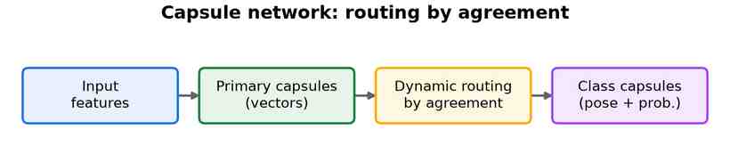
A capsule network was proposed to fix a specific weakness of convolutional networks: pooling throws away where a feature is and how it is oriented. A capsule outputs a small vector instead of a single number, encoding a feature's pose (position, orientation, scale) alongside its presence. Lower capsules then send their output to whichever higher capsule they agree with, a process called routing by agreement, sketched in Fig 10.

Origins and rise

Sabour, Frosst, and Hinton introduced dynamic routing between capsules in 2017, with a matrix-capsule variant following soon after.^[113] The idea is elegant and viewpoint-robust on small datasets, but the routing procedure is slow and has not yet scaled to the large benchmarks where convolutional and Transformer models dominate, so it remains largely a research direction.

Routing by agreement

The defining question for the family is how a lower capsule decides which higher capsule should receive its output. The original CapsNet answered with dynamic routing: it measures the agreement between a capsule's prediction and each candidate parent and iteratively strengthens the couplings that agree, squashing each vector's length to encode how confident it is that the feature is present.^[113] Matrix capsules replaced this with a more principled scheme: each capsule carries a 4×4 pose matrix and a separate activation, and routing is cast as expectation-maximization clustering, with lower capsules acting as data points assigned to the higher capsules that behave like Gaussian clusters.^[114] EM routing made the geometry of pose explicit and improved robustness to viewpoint and adversarial changes, at the cost of a delicate procedure that is slow to train.

Deeper and more efficient capsules

Both routing schemes were first demonstrated on shallow networks over small images, and stacking many capsule layers proved hard because iterative routing is expensive and its gradients are noisy. DeepCaps tackled this by building a deeper capsule network around 3D convolutional routing, trimming the parameter count while pushing capsule accuracy past the original on CIFAR-scale benchmarks.^[115] It stands for a broader effort to keep the pose-aware inductive bias of capsules while borrowing the depth and efficiency that let convolutional and Transformer backbones scale.

Unsupervised and 3D capsules

Later work moved capsules beyond supervised image classification. Stacked capsule autoencoders turn the idea inside out: instead of routing by agreement they infer object capsules and their parts with no labels at all, reconstructing an image as a composition of part templates and reading out the discovered capsules for strong unsupervised classification.^[116] The pose machinery also transfers naturally to geometry: 3D point capsule networks apply capsules to unordered point clouds, learning latent capsules that capture the parts of a shape for reconstruction, interpolation, and part segmentation.^[117] Together these variants show the family is less a single architecture than a recurring bet that explicit part–whole structure is worth modelling.

Applications

• Viewpoint-robust recognition on small image datasets.
• Medical-imaging research where part-whole structure matters.
• A testbed for ideas about pose and equivariance.

Strengths and limitations

Strengths	Limitations
Encode pose and part-whole relationships.	Routing is computationally slow.
Robust to viewpoint changes.	Have not scaled to large datasets.
Need fewer examples on simple tasks.	Still mainly a research architecture.

9. Siamese & Metric Learning Networks

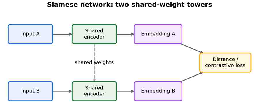
A Siamese network is less a new layer than a new training setup: two (or three) identical towers with shared weights encode their inputs into a common space, and the network is trained so that similar inputs land close together and dissimilar ones far apart, as in Fig 11. The towers themselves are usually convolutional or Transformer encoders; what makes the family distinct is the metric-learning objective.

Origins and rise

The design dates to Bromley and colleagues' signature-verification network in 1993,^[118] and reached maturity with FaceNet, whose triplet loss learned face embeddings good enough for verification at scale.^[119] The same contrastive idea now powers self-supervised pre-training and cross-modal models such as the vision-language systems later in this tree.

Contrastive losses: pairs, triplets, and structure

What sets the family apart is the loss, and its history is a march toward using more of each batch. The original contrastive loss operated on pairs, pulling matching examples together and pushing non-matching ones apart beyond a fixed margin.^[120] The triplet loss popularized by FaceNet compares an anchor against one positive and one negative at once, sidestepping the need to calibrate an absolute distance.^[119] Because most triplets become uninformative once training gets going, structured losses such as lifted structured embedding use every positive and negative pair within a mini-batch, folding hard-negative mining into the objective rather than a preprocessing step.^[121]

Metric-based few-shot learning

A natural use of a learned metric is recognizing new classes from a handful of examples. Matching Networks cast one-shot classification as a differentiable nearest-neighbour lookup over a small support set, trained episodically to mirror the test conditions.^[122] Prototypical Networks pared this down to a single prototype per class — the mean of its support embeddings — and classify by distance to those prototypes.^[123] Relation Networks go a step further and learn the comparison itself, replacing a fixed distance with a small network that scores how well a query matches each class.^[124] The optimization-based cousins of these methods sit with the meta-learning family later in this tree.

Self-supervised representation learning

The same twin-tower recipe, applied without labels, became an engine of modern representation learning. SimCLR showed that strong augmentation, a projection head, and a large batch of in-batch negatives suffice to learn features that rival supervised pre-training.^[125] MoCo removed the need for huge batches with a momentum-updated encoder and a queue of negatives.^[126] Then came a surprise: BYOL and SimSiam dropped negatives entirely, avoiding collapse with a predictor and a stop-gradient instead of contrastive pushing.^[127][128] SwAV swapped explicit pairs for online cluster-assignment matching,^[129] while Barlow Twins and VICReg prevent collapse by regularizing the statistics of the embeddings — decorrelating feature dimensions, or controlling their variance and covariance.^[130][131] On vision Transformers the same instinct surfaces as the self-distillation of DINO.^[64]

Deep metric learning for retrieval

For search and face recognition the goal is an embedding whose distances rank correctly, and two strands dominate. Margin-softmax losses reshape ordinary classification into an angular metric: ArcFace, alongside its sibling CosFace, adds a fixed margin on the hypersphere so that same-identity embeddings cluster tightly, setting the standard for face recognition.^[132] The other strand refines pairwise training: proxy methods such as Proxy Anchor learn a few representative points to compare against, cutting the cost of mining real pairs,^[133] while Multi-Similarity and Circle Loss weight each pair by how informative it is, unifying many earlier losses under a single view of pair-similarity optimization.^[134][135]

Applications

• Face and signature verification, and biometric matching.
• One-shot and few-shot recognition.
• Image retrieval and self-supervised representation learning.

Strengths and limitations

Strengths	Limitations
Work with very few labels per class.	Need careful pair or triplet sampling.
Add new classes without retraining.	Embedding quality rides on the encoder.
Ideal for verification and retrieval.	Training can collapse without the right loss.

10. Neural Differential Equations

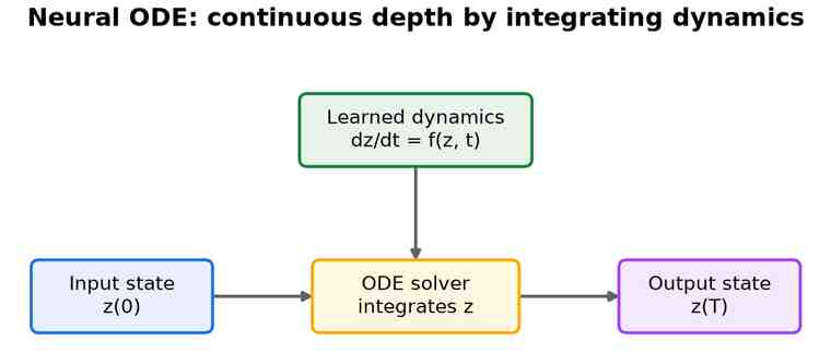
A neural ordinary differential equation (ODE) treats network depth as continuous. Instead of stacking a fixed number of discrete layers, it defines how the hidden state changes — its derivative — and hands that to an ODE solver to integrate from input to output, as in Fig 12. A residual network turns out to be a coarse, discrete version of exactly this — one Euler step per layer. The ODE formulation provides a natural way to adapt the number of function evaluations to the complexity of the problem, a property known as adaptive computation.

Origins and rise

Chen and colleagues introduced neural ODEs in 2018, training them memory-efficiently by solving a second, adjoint equation backwards.^[136] The framework extends naturally to continuous-time data and to generative normalising flows, and it links deep learning to a century of numerical-analysis tools.

Continuous-depth models and their limits

The original neural ODE recast a deep stack as the integral of a learned vector field,^[136] but that continuity carries a catch: because ODE trajectories cannot cross, a single neural ODE cannot represent some mappings a residual network handles with ease. Augmented neural ODEs resolve this by adding extra dimensions to the state, giving the trajectories room to flow around one another, which improves both expressivity and training stability.^[137]

Continuous-time models for irregular data

A key payoff of the framework is native handling of data that arrives at irregular times, where discrete recurrent networks must awkwardly bin or interpolate. Latent ODEs pair a recurrent encoder with an ODE that evolves a latent state in continuous time, so an observation at any timestamp slots in naturally.^[138] Neural controlled differential equations go further, driving the dynamics with an interpolated path of the incoming data — a continuous-time analogue of the RNN that inherits the mathematics of controlled differential equations and copes gracefully with partially observed streams.^[139]

Stochastic dynamics and continuous flows

The same machinery reaches from deterministic ODEs into probability and randomness. FFJORD turns a neural ODE into a continuous normalising flow, using an unbiased trace estimator so that exact likelihoods can be computed without the architectural constraints earlier flows imposed.^[140] Replacing the ODE with a stochastic differential equation adds a noise term: neural SDEs learn both a drift and a diffusion, trained with an adjoint sensitivity method that scales to many parameters,^[141] and casting such an SDE as the generator of a GAN yields a principled continuous-time generative model for time series.^[142]

Applications

• Irregularly sampled time series and continuous-time modelling.
• Continuous normalising flows for generative modelling.
• Physics- and dynamics-aware scientific models.

Strengths and limitations

Strengths	Limitations
Constant memory via the adjoint method.	The ODE solver makes training slow.
Adapt computation to the problem's difficulty.	Can be numerically stiff or unstable.
Natural fit for continuous-time data.	Often outperformed by simpler nets on plain tasks.

11. Spiking Neural Networks (SNN)

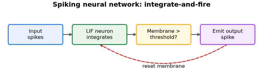
A spiking neural network is the family closest to the biology the introduction invoked. Its neurons communicate not with continuous numbers but with discrete spikes over time: a LIF neuron integrates incoming spikes until its membrane potential crosses a threshold, fires a spike, and resets, as in Fig 13. Computation is therefore sparse and event-driven. The dynamics of a LIF neuron can be described by the differential equation τ dV/dt = - (V - V_rest) + R I(t), where V is the membrane potential, τ is the time constant, and I(t) is the input current. When V exceeds a threshold, a spike is emitted and the potential resets.

Origins and rise

Maass framed spiking neurons as a “third generation” of network models in 1997.^[143] Because a spike is not differentiable, training was long the obstacle; the modern answer is the surrogate gradient, which substitutes a smooth approximation during backpropagation.^[144] Interest has grown alongside neuromorphic hardware, and many spiking models are obtained by converting a trained convolutional network.

Neuron models

How faithfully a spiking neuron mimics biology is a design choice. The leaky integrate-and-fire neuron of Fig 13 keeps only the essentials — leak, integrate, threshold, reset — and dominates practical work for its simplicity. The Izhikevich model adds a second recovery variable and, for only a handful of operations per step, reproduces the rich firing patterns of cortical neurons: bursting, chattering and adaptation.^[145] The adaptive exponential integrate-and-fire (AdEx) neuron sits between the two, pairing an exponential spike-initiation term with an adaptation current, and matches real recordings closely enough to serve as a workhorse in large-scale simulations.^[146]

Spike-timing-dependent plasticity

The oldest way to train a spiking network borrows a rule from neuroscience: spike-timing-dependent plasticity (STDP) strengthens a synapse when a presynaptic spike arrives just before a postsynaptic one and weakens it otherwise, learning from local timing alone with no global error signal. Diehl and Cook showed that a two-layer network trained this way, entirely unsupervised, recognises handwritten digits at competitive accuracy — an existence proof that biologically local learning scales beyond toy problems.^[147] Its appeal is hardware-friendliness — the update is local and needs no backward pass — but it has been hard to push to the depths gradient training reaches.

Converting trained networks to spikes

A pragmatic shortcut sidesteps spiking training altogether: train an ordinary convolutional network with real-valued activations, then convert it into a spiking one whose firing rates approximate those activations. Rueckauer and colleagues formalised the recipe — rescaling weights and thresholds so a rate-coded spiking network matches the original's accuracy — and extended it to the operations, such as max-pooling and batch normalisation, that real networks depend on.^[148] Sengupta and colleagues then scaled conversion to deep VGG and residual networks on ImageNet, closing much of the accuracy gap to the source model.^[149] Conversion buys accuracy at the price of latency, since firing rates need many timesteps to settle.

Surrogate-gradient training and deep spiking networks

Training a spiking network directly means confronting the non-differentiable spike, and the modern answer — the surrogate gradient introduced above — replaces the threshold's derivative with a smooth stand-in so that backpropagation through time can flow.^[144] SLAYER made this practical by also distributing the credit for an error backwards across time, accounting for a spike's delayed influence on the ones that follow.^[150] Scaling the idea deep required taming the firing statistics: a threshold-dependent batch normalisation let directly trained networks reach residual depths without the signal vanishing or saturating.^[151] Spikformer carried the approach into the Transformer era, recasting self-attention in a purely spike-driven, multiplication-free form.^[152]

Recurrent spiking networks and neuromorphic hardware

Because spikes unfold in time, a spiking network is inherently recurrent, and adding explicit feedback plus slow adaptation yields memory rivalling an LSTM: the LSNN equips neurons with an adapting threshold and learns tasks that demand holding information across many timesteps.^[153] The payoff for all this is energy, realised on neuromorphic hardware that computes only when spikes occur. IBM's TrueNorth packed a million spiking neurons onto a chip drawing tens of milliwatts,^[154] and Intel's Loihi added on-chip plasticity so that STDP-style learning can run in silicon.^[155] These chips are the reason the family is pursued despite trailing standard networks on raw accuracy.

Applications

• Ultra-low-power inference on neuromorphic chips such as Loihi and TrueNorth.
• Event-camera and always-on sensing at the edge.
• Computational-neuroscience models of the brain.

Strengths and limitations

Strengths	Limitations
Very energy-efficient on neuromorphic hardware.	Non-differentiable spikes are hard to train.
Naturally encode timing and events.	Tooling and hardware are still immature.
Biologically plausible.	Often trail standard networks on accuracy.

12. Attention Plug-in Modules

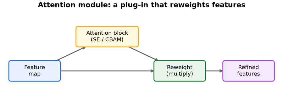
Not every use of attention is a full Transformer. A family of lightweight attention modules exists to be bolted on to an existing convolutional network, letting it reweight its own features by importance. As Fig 14 shows, the module looks at a feature map, computes a set of weights, and multiplies them back in to emphasise the informative channels or locations.

Origins and rise

Squeeze-and-Excitation networks won the 2017 ImageNet challenge by recalibrating channels with a tiny attention branch,^[156] and the convolutional block attention module (CBAM) added spatial attention on top the following year.^[157] They are conceptual cousins of the Transformer's self-attention and of the neighbour weighting in graph attention.

Channel attention

The simplest question an attention module can ask is which channels matter. Squeeze-and-Excitation, introduced above, answers it by pooling each channel to a single number, learning a per-channel gate from that summary, and rescaling the feature map.^[156] ECA-Net shows the small fully-connected bottleneck SE uses to mix channels is unnecessary: a cheap one-dimensional convolution over neighbouring channels captures the same cross-channel interaction with a handful of extra parameters.^[158] Selective Kernel networks add a second axis of choice, attending over branches with different receptive-field sizes so the network adapts its effective kernel to the scale of the object in view.^[159]

Adding spatial attention

Channels say what; pixels say where. The convolutional block attention module (CBAM), noted above, chains a channel gate with a spatial one so the network learns both which features and which locations to emphasise.^[157] BAM arranges the same two attentions in parallel rather than in sequence and places the combined module at the network's bottlenecks, where downsampling makes feature selection most valuable.^[160]

Capturing long-range context

Convolution is local by construction, so a distant but relevant pixel influences another only after many layers. The non-local block borrows the Transformer's idea directly, computing the response at each position as a weighted sum over all positions and capturing long-range dependencies in a single step.^[161] Its cost is quadratic in the number of pixels, which spurred cheaper variants: GCNet observed that the non-local attention map is nearly identical for every query and collapsed it into a single shared context, fusing the thrift of Squeeze-and-Excitation with the reach of the non-local block.^[162] CCNet instead gathers context along criss-cross paths — each pixel attends only to its own row and column — and recovers full-image coverage by stacking two such passes, cutting the cost sharply for dense prediction.^[163]

Self-attention as a convolution replacement

A more radical step replaces convolution outright. Stand-alone self-attention swaps every spatial convolution in a residual network for a local self-attention layer, showing a vision backbone can be built from attention alone.^[164] Because full two-dimensional attention is expensive, axial attention factorises it into attention along rows followed by attention along columns; Axial-DeepLab builds a panoptic-segmentation backbone on this decomposition, reaching a large receptive field at manageable cost.^[165] These modules foreshadow the vision Transformer, which abandons the convolutional backbone entirely.

Applications

• Drop-in accuracy boosts for classification and detection backbones.
• Efficient mobile and embedded vision models.
• Any convolutional pipeline that benefits from sharper feature selection.

Strengths and limitations

Strengths	Limitations
Cheap, plug-and-play accuracy gains.	Improvements are incremental, not transformative.
Add few parameters.	Add some latency to every forward pass.
Work with almost any backbone.	Not a standalone architecture.

13. Neural Architecture Search (NAS)

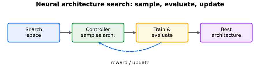
Neural architecture search automates the design of the network itself. Rather than a human choosing how many layers of what kind to stack, a search process proposes architectures from a defined space, trains and evaluates them, and uses the result to propose better ones, as the loop in Fig 15 makes clear. Several of the strongest convolutional backbones were discovered this way.

Origins and rise

Zoph and Le framed the search as a reinforcement-learning problem in 2017, with a controller rewarded for proposing accurate networks.^[166] That was powerful but hugely expensive; DARTS made the search differentiable, relaxing the discrete choice of operations into a continuous one solvable by gradient descent.^[167] Discovered models such as MnasNet and EfficientNet followed.

Cell-based and weight-sharing search

The reinforcement-learning controller was made practical by two ideas. NASNet searched not for a whole network but for a small cell — a reusable block — on a small proxy dataset, then stacked copies of it to any depth, so a search run on CIFAR-10 transferred to ImageNet.^[168] Even so, every candidate still had to be trained from scratch. ENAS removed that cost by forcing all candidates to share one set of weights, treating each as a subgraph of a single over-parameterised network, and collapsed the search from thousands of GPU-days to less than one.^[169]

Differentiable search

DARTS recast the discrete choice of operation on each edge as a weighted mixture, making the whole architecture differentiable and solvable by gradient descent^[167] — but the relaxation is fragile. PC-DARTS sampled only a fraction of the channels on each edge, cutting the memory that had confined searches to tiny proxies,^[170] while P-DARTS grew the network's depth progressively so the searched and evaluated architectures finally matched.^[171] Two later fixes tackled a notorious failure mode in which the search collapses onto parameter-free skip connections: Fair DARTS removed the unfair advantage those connections enjoy,^[172] and DARTS‑ stepped out of the collapse without hand-tuned indicators.^[173]

Hardware-aware search

Efficiency on a real device depends on more than parameter count, so the reward itself was made hardware-aware. MnasNet folded measured on-phone latency directly into a multi-objective reward, yielding mobile models on the accuracy-latency frontier,^[174] and MixNet then let a single searched layer mix several depthwise kernel sizes at once.^[175] On the differentiable side, ProxylessNAS searched directly on the target task and hardware rather than a proxy, modelling latency as a differentiable loss,^[176] and FBNet steered a DARTS-style search toward a specific chip with a latency lookup table.^[177] The same principle carried to language, where HAT searched hardware-aware transformer configurations tuned to the latency of the deployment device.^[178]

Train-once supernets

Searching afresh for every deployment target is wasteful when many targets share one problem. Once-for-All trained a single elastic supernet from which specialised sub-networks of differing depth, width, and resolution can be extracted for any latency budget without retraining,^[179] and BigNAS pushed the idea further, training one big single-stage model whose sliced sub-networks are deployment-ready as sampled.^[180] Making weight sharing fair is delicate, however: SCARLET-NAS stabilised supernet training so that a candidate's shared-weight accuracy actually predicts its stand-alone accuracy.^[181]

Searching beyond convolutions

Search need not stop at convolutional cells. AutoFormer applied weight-sharing search to vision transformers, entangling the weights of candidate blocks so that thousands of sub-transformers could be ranked from one supernet.^[182] The field's impact is clearest, though, in the backbones now in everyday use: EfficientNet paired a searched mobile block with compound scaling,^[18] while RegNet searched over design spaces rather than individual networks, distilling the outcome into simple, quantised rules for width and depth.^[183]

Applications

• Designing efficient image backbones under size or latency budgets.
• Hardware-aware models tailored to a specific chip.
• Automating model design where expert tuning is scarce.

Strengths and limitations

Strengths	Limitations
Automates a slow, expert-driven process.	Early methods needed enormous compute.
Can beat hand-designed networks.	The search space is still designed by hand.
Optimises directly for the target hardware.	Results can be hard to reproduce.

14. Reinforcement Learning Network Architectures

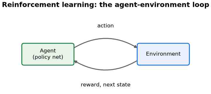
Reinforcement learning (RL) is a training paradigm rather than a single architecture: an agent learns by trial and error to take actions that maximise long-term reward in an environment, the loop shown in Fig 16. The agent's policy and value functions are neural networks — typically feedforward or convolutional nets when the input is pixels.

Origins and rise

Deep RL arrived in 2015 when the deep Q-network (DQN) learned to play Atari games directly from pixels at human level.^[184] Policy-gradient methods such as PPO then made training more stable and became the workhorse for continuous control.^[185] The same machinery drives the reinforcement-learning-from-human-feedback step that aligns modern Transformer language models, and it powered the controllers behind early architecture search.

Value-based methods

The DQN template — a network that estimates the value of each action, trained on replayed experience^[184] — was sharpened by a rapid succession of fixes. Double DQN corrected the systematic over-estimation of action values,^[186] and the dueling architecture split the network into separate state-value and advantage streams.^[187] A parallel line replaced the single value estimate with a whole distribution over returns: C51 modelled that distribution on a fixed support,^[188] QR-DQN learned its quantiles directly,^[189] and IQN sampled them implicitly for a fuller picture of risk.^[190] Rainbow showed these gains are complementary, folding six of them into one agent,^[191] while Ape-X scaled learning across hundreds of actors feeding one prioritised replay buffer.^[192]

Policy-gradient and actor-critic methods

Where value-based agents suit discrete actions, policy-gradient methods optimise the policy directly and handle continuous control. A3C ran many actor-learners asynchronously to decorrelate their updates,^[193] and TRPO made large policy steps safe by constraining each update to a trust region^[194] — a constraint that PPO later approximated with a simple clipped objective.^[185] For continuous action spaces, DDPG carried the deterministic-policy idea into deep networks,^[195] TD3 curbed its value over-estimation with twin critics and delayed updates,^[196] and SAC added an entropy bonus that rewards exploration, becoming a robust default for robotics.^[197]

Model-based agents and world models

Model-free agents are notoriously sample-hungry, so a complementary strand learns a model of the environment and plans inside it. The World Models proposal trained a compact recurrent latent model and let a tiny controller learn entirely inside its imagined rollouts.^[198] PlaNet planned directly from pixels through a learned latent dynamics model,^[199] and the Dreamer line scaled this into a general agent that learns behaviours by imagining rollouts, with DreamerV3 mastering diverse domains under one fixed set of hyper-parameters.^[200] A different branch plans with a learned model of reward and value rather than pixels: MuZero reached superhuman play in Go, chess, shogi, and Atari without being told the rules,^[201] and EfficientZero brought that approach to human-level Atari from roughly two hours of experience.^[202]

Multi-agent architectures

When several agents share an environment, each one's learning shifts the others' world, so specialised architectures stabilise the joint problem. MADDPG gave each agent a centralised critic that sees every agent's actions while it still acts on local observations.^[203] For cooperative teams with a single shared reward, value-decomposition methods learn how to credit individuals: VDN summed per-agent values,^[204] QMIX generalised this to a monotonic mixing network,^[205] and COMA used a counterfactual baseline to isolate each agent's contribution.^[206] More recently, MAPPO showed that PPO paired with a centralised critic is a surprisingly strong baseline for these cooperative games.^[207]

Applications

• Game playing, from Atari and Go to real-time strategy.
• Robotics, control, and operations research.
• Aligning language models through human feedback.

Strengths and limitations

Strengths	Limitations
Learn from interaction, without labelled data.	Very sample-inefficient.
Optimise long-term, delayed goals.	Training can be unstable and hard to reproduce.
Reach superhuman play in many games.	Designing the reward is subtle and error-prone.

15. Multimodal & Vision-Language

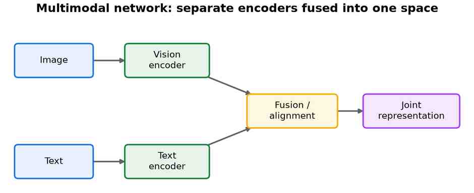
A multimodal network handles more than one kind of input at once — most often images together with text. The standard recipe, in Fig 17, encodes each modality with its own network — a convolutional or vision Transformer for images, a Transformer for text — and then fuses or aligns the two representations into a shared space.

Origins and rise

CLIP aligned images and captions with a contrastive objective — the same metric-learning idea applied across modalities — and unlocked zero-shot classification from natural-language labels.^[208] Flamingo then showed few-shot visual question answering by feeding image features into a frozen language model.^[209] The same encoders feed the generative text-to-image systems that turn a prompt into a picture.

Image-text alignment

CLIP's contrastive recipe^[208] was quickly scaled and refined. ALIGN showed that a noisy billion-scale web dataset could stand in for careful curation,^[210] LiT found that locking a pre-trained image encoder while tuning only the text tower gives stronger zero-shot transfer,^[211] and SigLIP swapped the softmax contrastive loss for a simple pairwise sigmoid that trains well even at small batch sizes.^[212]

Fusion encoders for question answering

Before contrastive pre-training, visual question answering was driven by attention over detected objects: the Bottom-Up and Top-Down model attended to region features from an object detector.^[213] The BERT era then produced Transformer encoders that fuse the two modalities directly: ViLBERT used two streams joined by cross-attention,^[214] LXMERT a comparable cross-modality encoder,^[215] and UNITER a single stream that concatenates image regions with word tokens.^[216]

Generative vision-language models

The next wave connected vision encoders to generative language models so the output is free-form text. BLIP bootstrapped noisy web captions to pre-train for both understanding and generation,^[217] and BLIP-2 bridged a frozen image encoder to a frozen large language model through a lightweight querying transformer.^[218] Flamingo interleaved image and text tokens for few-shot prompting,^[209] while PaLI jointly scaled the vision and language towers across many languages.^[219]

Visual grounding

Grounding models tie phrases to specific image regions. MDETR extended the DETR detector^[23] to condition detection on a free-text query,^[220] and Grounding DINO married a strong detector with grounded pre-training for open-set detection from arbitrary prompts.^[221] Kosmos-2 folded grounding into a multimodal language model, letting it point to regions as it generates text.^[222]

Document understanding

A specialised branch reads text-rich images such as forms, receipts, and screenshots. LayoutLMv3 jointly masks text and image patches to learn layout-aware representations,^[223] while Donut reads documents OCR-free, decoding structured output straight from pixels.^[224] Pix2Struct pre-trained by parsing masked webpage screenshots, transferring to charts, user interfaces, and diagrams.^[225]

Unified any-task models

The frontier folds every task into one sequence-to-sequence model. CoCa trained a single network under both contrastive and captioning objectives,^[226] and Unified-IO cast vision, language, and dense prediction tasks into one shared token vocabulary.^[227] BEiT-3 treated images as another language to pre-train a shared backbone across vision and vision-language tasks,^[228] and ImageBind learned a single embedding space binding six modalities using only image-paired data.^[229]

Applications

• Text-to-image retrieval and zero-shot classification.
• Visual question answering, captioning, and document understanding.
• Open-vocabulary detection and multimodal assistants.

Strengths and limitations

Strengths	Limitations
Transfer to new tasks with no fine-tuning.	Need enormous paired image-text datasets.
One model spans several modalities.	Inherit and can amplify dataset biases.
Enable open-vocabulary, language-driven tasks.	Expensive to train and to serve.

16. Recommendation & Retrieval Networks

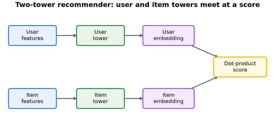
A recommender predicts which items a user is likely to engage with. The dominant modern design is the two-tower retrieval network in Fig 18: a user tower and an item tower each map their features into the same embedding space, and relevance is simply the dot product of the two embeddings — so millions of candidate items can be scored by fast nearest-neighbour search.

Origins and rise

Wide & Deep paired a memorising linear model with a generalising deep network.^[230] Neural Collaborative Filtering replaced the classic matrix-factorisation dot product with a learned network over user and item embeddings,^[231] and DLRM scaled the recipe to industrial click-through prediction with enormous embedding tables.^[232]

Modelling feature interactions

A click-through model lives or dies on how well it combines sparse categorical features, so a family of models extends the Wide & Deep template^[230] with explicit interaction machinery. DeepFM fused a factorisation machine with a deep network over a shared embedding table, learning low- and high-order feature crosses jointly.^[233] Deep & Cross Network replaced the memorising wide side with a cross network that builds bounded-degree feature crosses at every layer,^[234] and its successor DCN V2 made those crossing matrices low-rank so they scale to web-scale ranking.^[235] xDeepFM added a compressed interaction network that crosses features at the vector rather than the bit level,^[236] while AutoInt used multi-head self-attention to learn automatically which feature combinations matter.^[237]

Sequential recommenders

Rather than treat a user as a static bag of preferences, sequential models predict the next item from the ordered history of interactions. GRU4Rec first applied a recurrent network to anonymous session data,^[238] then SASRec swapped the recurrence for a causal self-attention stack that captures long-range dependencies more cheaply.^[239] BERT4Rec made the attention bidirectional, training with a masked-item objective borrowed from BERT,^[240] and SR-GNN modelled each session as a graph, propagating with a graph neural network to capture more complex item transitions.^[241]

Two-tower retrieval

At web scale a model cannot score every item for every request, so candidate retrieval is split into two independent encoders like those in Fig 18. DSSM introduced this design for web search, mapping queries and documents into a shared semantic space where relevance is a cosine similarity.^[242] The YouTube recommender scaled the idea to hundreds of millions of videos with a deep candidate-generation tower whose output embeddings are served by approximate nearest-neighbour search,^[243] the factorisation that lets the item tower be precomputed and indexed offline.

Applications

• Product, video, and feed recommendation at web scale.
• Advertising click-through and conversion prediction.
• Candidate retrieval via approximate nearest-neighbour search.

Strengths and limitations

Strengths	Limitations
Score millions of items via precomputed embeddings.	Cold start: little signal for new users or items.
Learn feature interactions automatically.	Sparse embedding tables dominate memory.
Decouple offline indexing from online serving.	Feedback loops can amplify popularity bias.

17. Point Cloud & 3D Data Networks

A point cloud is an unordered set of 3-D points — the raw output of a LiDAR sensor or depth camera — so the network must give the same answer whatever order the points arrive in. PointNet, in Fig 19, solves this by applying a shared MLP to every point independently and then collapsing them with a symmetric max-pool into a single global descriptor. The architecture is a direct application of the set-invariant principle, and its success demonstrated that deep learning on raw point clouds is possible without the explicit structure of a grid.

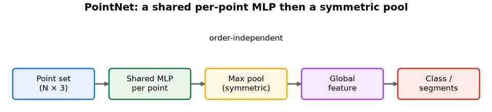
Origins and rise

PointNet introduced the shared-MLP-plus-symmetric-pooling recipe.^[244] PointNet++ added hierarchical local grouping so the model could capture fine geometry, not just a global summary.^[245] A different line, neural radiance fields (NeRF), fits a small network mapping a 3-D coordinate and viewing direction to colour and density, rendering photorealistic novel views.^[246]

Convolutions on points

A global max-pool discards local geometry, so a family of models redefines convolution to act on an irregular neighbourhood of points. PointCNN learns an X-transformation that reorders and weights local points before a standard convolution, recovering the exploitation of spatial layout.^[247] PointConv treats the convolution kernel as a continuous function of relative position, approximated by an MLP and reweighted by the local density so it can be applied at any coordinate.^[248] KPConv instead places a set of learnable kernel points in space, letting each carry a weight that deforms to the local geometry.^[249] SpiderCNN parameterises its filters as a family of polynomial functions over neighbours,^[250] and PAConv assembles each kernel dynamically by mixing a learned weight bank with coefficients predicted from point positions.^[251] Countering this trend, PointMLP showed that a plain residual MLP with a geometric affine module rivals these operators, suggesting elaborate local extractors are not strictly necessary.^[252]

Graph-based point networks

Because a point cloud is naturally a neighbourhood graph, some models borrow directly from graph neural networks. Dynamic Graph CNN introduced EdgeConv, which builds a k-nearest-neighbour graph in feature space and recomputes it at every layer, so points that are semantically — not just spatially — close exchange information.^[253] This dynamic recomputation lets the receptive field follow the shape's structure rather than a fixed spatial radius.

Point transformers

Self-attention is permutation-invariant by construction, making it a natural fit for unordered points. Point Cloud Transformer and Point Transformer both apply attention within local neighbourhoods, the latter using vector attention so each channel is weighted independently.^[254][255] Stratified Transformer samples distant points sparsely and nearby points densely as attention keys, capturing long-range context for scene segmentation without quadratic cost,^[256] while OctFormer uses an octree to sort points into windows of equal count, making attention scale to millions of points.^[257]

Voxel and sparse-convolution backbones

A complementary route rasterises points into a 3-D grid so ordinary convolution applies. VoxNet was an early dense-voxel CNN for real-time object recognition,^[258] but a dense grid wastes computation on empty space. Submanifold sparse convolution fixes this by storing and convolving only occupied voxels, keeping the active sites sparse,^[259] and MinkowskiNet generalised sparse convolution to arbitrary dimensions, enabling high-resolution 4-D spatio-temporal networks.^[260] For autonomous driving, SECOND brought sparse convolution to LiDAR object detection, greatly speeding up the voxel backbone.^[261]

Implicit neural fields

Rather than store geometry as points or voxels, implicit models represent a shape as a continuous function learned by a network — a decoder in the spirit of the generative families. DeepSDF regresses the signed distance to the surface from any 3-D coordinate, so a whole class of shapes is compressed into one conditioned network.^[262] Occupancy Networks predict instead whether a point lies inside or outside the object, giving a watertight surface at any resolution.^[263] Convolutional Occupancy Networks add local convolutional features so the representation scales from single objects to whole scenes.^[264]

Registration and odometry

Aligning two overlapping scans is the classical registration problem, and learned methods now replace hand-tuned iterative closest point. PointNetLK unrolls a Lucas–Kanade alignment on PointNet global features, back-propagating through the optimisation steps.^[265] Deep Closest Point matches learned per-point features with attention and solves for the rigid transform in closed form,^[266] and RPM-Net adds a learned annealing that makes matching robust to noise and partial overlap.^[267] PointDSC then prunes wrong correspondences by enforcing spatial consistency, sharpening the final alignment.^[268]

Applications

• LiDAR perception for self-driving cars and robotics.
• 3-D shape classification, part segmentation, and registration.
• Novel-view synthesis and 3-D scene reconstruction.

Strengths and limitations

Strengths	Limitations
Operate directly on raw points, no voxelisation.	Global pooling can miss fine local structure.
Permutation-invariant by construction.	Scale poorly to very large scenes.
Compact and fast to run.	Sensitive to sampling density and noise.

18. Temporal Convolutional & Time-Series Networks

Sequences do not have to be processed with recurrence. A temporal convolutional network (TCN) stacks dilated causal convolutions, shown in Fig 20, whose receptive field grows exponentially with depth — so each output can look far into the past while, unlike an RNN, every time step is computed in parallel.

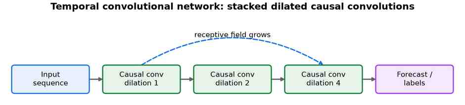
Origins and rise

Bai, Kolter & Koltun showed that a generic TCN matches or beats LSTMs across a wide range of sequence benchmarks.^[269] For forecasting specifically, N-BEATS stacked fully connected blocks with a basis-expansion structure,^[270] and Informer made the Transformer efficient for long-horizon time series with a sparse attention mechanism.^[271]

Dilated-convolution forecasters

The dilated causal stack that defines the TCN predates it: WaveNet introduced dilated causal convolutions to generate raw audio sample by sample, and the same structure underlies the general-purpose TCN.^[87] SCINet refines the convolutional route for forecasting: it repeatedly downsamples the series into odd and even sub-sequences and lets them interact, so each convolution sees several temporal resolutions at once.^[272]

Specialised forecasting networks

A line of purpose-built forecasters extends the basis-expansion idea of N-BEATS.^[270] N-HiTS adds multi-rate sampling and hierarchical interpolation, cutting the cost of long-horizon forecasts while improving accuracy.^[273] Where those give point forecasts, DeepAR trains an autoregressive recurrent network to output the parameters of a probability distribution, producing calibrated uncertainty across thousands of related series.^[274] MQRNN instead predicts a set of quantiles directly for every future step, giving multi-horizon prediction intervals in a single pass.^[275] Temporal Fusion Transformer combines recurrent encoding, variable-selection networks, and interpretable attention to mix static, known-future, and observed inputs in one model.^[276]

Transformers for long-horizon forecasting

After Informer made long-range attention tractable,^[271] a wave of Transformer forecasters targeted the structure of time series directly. Autoformer replaces dot-product attention with an auto-correlation mechanism and an internal series-decomposition block,^[277] and FEDformer moves the mixing into the frequency domain for a linear-complexity attention.^[278] PatchTST showed that splitting each channel into sub-series patches and treating channels independently gives a simple, strong baseline,^[279] while TimesNet reshapes a 1-D series into 2-D tensors along discovered periods so ordinary convolution captures both intra- and inter-period variation.^[280]

Time-series anomaly detection

Detecting anomalies in multivariate telemetry is usually framed as unsupervised reconstruction: a model learns normal dynamics and flags what it cannot reproduce. USAD pairs two autoencoders in an adversarial game so reconstruction is sensitive to subtle deviations,^[281] TranAD uses a lightweight Transformer with adversarial training and fast meta-learning to score deviations across many channels,^[282] and the Anomaly Transformer exploits an association-discrepancy criterion — anomalies attend locally while normal points attend globally — to separate the two.^[283]

Applications

• Demand, energy, and financial forecasting.
• Anomaly detection in sensor and system telemetry.
• Long causal sequences where parallel training matters.

Strengths and limitations

Strengths	Limitations
Parallel training with stable gradients.	Receptive field is fixed at design time.
Long memory through dilation.	Long horizons need many layers or wide kernels.
A simple, strong forecasting baseline.	Less flexible than attention for irregular sampling.

19. Set & Permutation-Invariant Networks

Some inputs are genuinely sets — a bag of items with no meaningful order. A permutation-invariant network, in Fig 21, encodes every element with a shared function, pools them with a symmetric operation such as sum or mean, then decodes the result; swapping two elements cannot change the output.

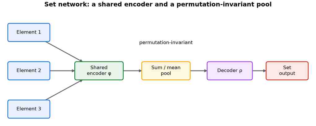
Origins and rise

Deep Sets proved that any permutation-invariant function can be written in this encode-pool-decode form, giving a clean sufficient condition: the element encoder must map into a latent space rich enough that summation there loses no information.^[284] The Set Transformer then replaced simple pooling with attention between the elements, capturing interactions a plain sum cannot represent.^[285] The same pooling idea underlies point-cloud and graph networks, and it is also the implicit backbone of modern aggregation in vision-language token pooling.

Beyond sum-pooling

A plain sum or mean is invariant but throws away how elements relate. Janossy Pooling spans the whole spectrum between the two extremes: it averages a permutation-sensitive function over orderings, and by restricting to k-ary sub-permutations it trades expressivity for cost — at k=1 it recovers sum-pooling, at full k it becomes an order-sensitive model averaged over all permutations.^[286] RepSet takes a geometric view, comparing each input set against learned hidden sets through a Hungarian bipartite-matching problem so the pooled representation reflects correspondence rather than mere co-occurrence.^[287] These designs are motivated by a theoretical limit: sum-pooling can represent any set function only if the latent dimension is at least the set size, so a small bottleneck provably loses information.^[288]

Predicting sets as output

Producing a set is harder than consuming one, because any fixed output ordering fights the target's permutation symmetry. Deep Set Prediction Networks sidestep this by predicting a set through an inner gradient-based optimisation whose loss is itself permutation-invariant.^[289] Slot Attention instead learns a small number of interchangeable slots that compete, via attention, to bind to parts of the input, giving an object-centric set representation that generalises across scenes with different object counts.^[290]

Applications

• Point-cloud and multi-object reasoning.
• Statistics and predictions over variable-size collections.
• Pooling inside graph and few-shot models.

Strengths and limitations

Strengths	Limitations
Exactly invariant to input order.	Simple pooling loses element interactions.
Handle variable-size inputs.	Attention pooling costs grow with set size.
Small and general-purpose.	Cannot represent order when it does matter.

20. Deep Equilibrium Models

A deep equilibrium model (DEQ) replaces a deep stack of layers with a single layer applied until it settles to a fixed point, where the output stops changing: z* = f(z*, x). As Fig 22 shows, a root-finding solver drives the iteration, and gradients come from implicit differentiation at the solution — so training uses constant memory no matter the effective depth.

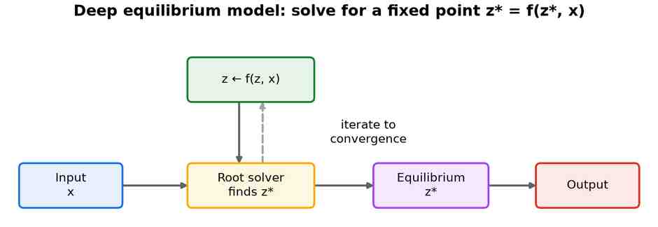
Origins and rise

Bai, Kolter & Koltun introduced DEQs, showing a single implicit layer can match a deep weight-tied network.^[291] Multiscale DEQ extended the idea to several resolutions at once, reaching competitive results on image classification and language modelling.^[292] Like neural ODEs, DEQs treat depth implicitly rather than as a fixed stack of layers.

Guaranteeing and stabilising equilibria

An implicit layer is only useful if its fixed point exists, is unique, and can be found reliably. Implicit Deep Learning set out the general framework, giving well-posedness conditions under which an equilibrium equation defines a valid layer.^[293] Monotone operator equilibrium networks made this constructive: by parameterising the layer as a monotone operator, they guarantee a unique fixed point reachable by a provably convergent solver.^[294] In practice DEQs can grow unstable as training proceeds, so Jacobian regularisation penalises the fixed-point Jacobian to keep the solver fast and the model well-conditioned.^[295]

Implicit models across domains

The equilibrium idea travels well beyond sequence models. Implicit graph neural networks solve for a fixed point of the message-passing update, behaving like an infinitely deep GNN that captures long-range dependencies a few explicit layers miss.^[296] Deep equilibrium optical flow solves directly for the flow field as the fixed point of an implicit refinement layer, matching recurrent estimators at a fraction of the training memory.^[297] This continuous, memory-light view of depth is shared with neural ODEs, which reach a solution by integrating a differential equation rather than by finding a fixed point.^[136]

Applications

• Memory-constrained sequence and vision models.
• Implicit graph neural networks.
• Very-deep behaviour without storing every layer.

Strengths and limitations

Strengths	Limitations
Constant training memory at any effective depth.	Each forward pass runs an iterative solver.
Backprop needs only the fixed point.	Convergence is not guaranteed.
Elegant and expressive.	Slower and less stable than explicit stacks.

21. Neuroevolution & Evolutionary Networks

Neuroevolution searches for networks without gradient descent. As Fig 23 shows, an evolutionary loop scores a population of networks by a fitness measure, keeps the best, and breeds the next generation by mutation and crossover — of the weights, and sometimes of the network topology itself.

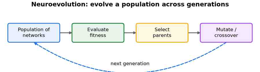
Origins and rise

NEAT evolved both weights and structure, growing networks from minimal seeds.^[298] HyperNEAT evolved a pattern that generates the weights of a much larger network.^[299] For deep reinforcement learning, Evolution Strategies showed a simple population-based optimiser can rival gradient methods while parallelising across thousands of workers.^[300]

Evolving topology and indirect encodings

NEAT's idea of evolving structure scales up in several directions. CoDeepNEAT coevolves reusable modules and the blueprints that wire them together, assembling deep networks in an evolutionary counterpart to architecture search.^[301] ES-HyperNEAT extends HyperNEAT's indirect encoding so evolution also decides where neurons sit and how densely they connect, rather than assuming a fixed substrate.^[302] EANT2 grows topologies incrementally while optimising each structure's weights with an evolution strategy, a combination well suited to control.^[303] Taking the idea to its limit, Weight Agnostic Neural Networks search for architectures that already perform a task when every weight shares a single random value, showing how much a topology alone can encode.^[304]

Rewarding novelty and scaling neuroevolution

A recurring failure of fitness-driven search is convergence to deceptive local optima. Novelty Search confronts this by abandoning the objective entirely and rewarding behaviours simply for being different, often reaching goals that direct optimisation cannot.^[305] On the scaling front, Deep Neuroevolution showed a plain genetic algorithm can train networks with millions of parameters for reinforcement learning, competitive with gradient-based methods and evolution strategies.^[306] Population Based Training blends the two paradigms, evolving a population of networks while they train by gradient descent so that hyperparameters are tuned online.^[307]

Applications

• Reinforcement-learning control without gradients.
• Evolving architectures, akin to architecture search.
• Black-box optimisation of non-differentiable objectives.

Strengths and limitations

Strengths	Limitations
Handle sparse, non-differentiable rewards.	Sample-inefficient: many evaluations needed.
Embarrassingly parallel across workers.	Compute-heavy at scale.
Can grow topology, escaping fixed designs.	Hard to tune and reproduce.

22. Meta-Learning & Few-Shot Architectures

Meta-learning aims to “learn to learn”: produce a model that adapts to a brand-new task from only a handful of examples. Optimisation-based methods use the bi-level loop in Fig 24 — an inner loop adapts to each task, while an outer loop updates a shared initialisation so that adaptation is fast.

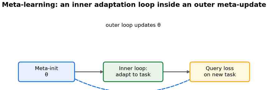
Origins and rise

MAML learned an initialisation from which a few gradient steps solve a new task,^[308] and Reptile reached similar results with a simpler first-order update.^[309] Metric-based methods such as Prototypical Networks instead classify by distance to per-class prototypes — the same metric-learning idea applied to few-shot problems.^[123]

Optimisation-based meta-learning

Optimisation-based methods, the family sketched in Fig 24, learn how to adapt rather than how to classify. MAML is the archetype: it learns an initialisation from which a few gradient steps on a new task reach a good solution,^[308] and Reptile reached the same end with a far simpler first-order update that avoids second-order derivatives.^[309] Meta-SGD goes further and meta-learns not just the initialisation but the learning rate and update direction for each parameter,^[310] while MetaOptNet replaces the inner gradient descent with a convex classifier such as a support-vector machine, casting few-shot learning as meta-learning a learner.^[311] When the model is too large to differentiate through directly, latent embedding optimisation (LEO) instead meta-learns in a low-dimensional latent space, recovering fast adaptation for big architectures.^[312]

Metric-based few-shot learning

Metric-based methods skip adaptation altogether and learn a comparison function, so a new class is recognised by its relation to a few labelled examples — an idea shared with the Siamese and metric-learning family. Matching Networks set the template by classifying a query with a soft nearest-neighbour vote over the support set,^[122] and Prototypical Networks simplified it to distance from a per-class prototype, the mean of its support embeddings.^[123] Relation Networks make that comparison itself learnable rather than fixing a Euclidean metric.^[124] A second thread leans on learned architectures rather than fixed metrics: the simple neural attentive meta-learner (SNAIL) embeds a temporal convolution and attention module that, given a short episode of labelled examples, learns to use them as context for the query.^[313]

Model-based meta-learning

Model-based methods encode the “how to learn” rule directly into the architecture — typically with external memory or weight generation. The memory-augmented neural network (MANN) stores labelled examples in an addressable external memory and reads from it at inference, so one-shot learning reduces to writing the new example and looking it up.^[314] More broadly, any HyperNetwork that generates a model's weights conditioned on the task can be read as model-based meta-learning — the idea formalised in the next family.^[315] These designs adapt in a single forward pass, which is faster than optimisation-based methods, but the learned strategy is less explicit and generalises less predictably to tasks unlike those seen in training.

Applications

• Few-shot image classification.
• Fast adaptation in robotics and personalisation.
• Learning initialisations and hyper-parameters.

Strengths and limitations

Strengths	Limitations
Adapt from only a few examples.	Bi-level training is expensive and finicky.
Task-agnostic initialisation.	Sensitive to task-distribution mismatch.
Bridge naturally to metric learning.	Struggle as tasks grow more complex.

23. HyperNetworks & Parameter-Efficient Tuning

Two related ideas treat a network's weights as something to generate or nudge cheaply. A hypernetwork is one network that outputs the weights of another. Parameter-efficient fine-tuning freezes a large pretrained model and trains a tiny add-on; LoRA, in Fig 25, adds a low-rank update B·A beside each frozen weight, so only a few million parameters are learned.

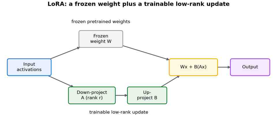
Origins and rise

HyperNetworks introduced the idea of one network generating another's weights.^[315] LoRA made low-rank adaptation the default way to fine-tune large language models,^[316] and QLoRA combined it with 4-bit quantisation to fine-tune very large models on a single GPU.^[317]

Weight-generating hypernetworks

The original HyperNetworks idea let an embedding condition the weights of a recurrent network, compressing many parameter sets into one generator.^[315] A related trick, dynamic convolution, generates several convolution kernels and mixes them by input-dependent attention, keeping a model compact yet expressive at runtime.^[318] The same generator-as-controller pattern underpins the model-based meta-learning networks that condition a learner on task context.

Adapter modules and bottleneck insertion

Adapters add small trainable modules between the layers of a frozen Transformer, the family sketched in Fig 25. The Houlsby adapter inserted a bottleneck module after every sub-layer and matched full fine-tuning with only a few percent of the parameters,^[319] while the Pfeiffer adapter showed that placing adapters only after the feed-forward block is almost as effective and more efficient. This spawned a long line of cross-task and cross-lingual adapter stacks that share one backbone.

Low-rank reparameterisation

LoRA reframed adaptation as a low-rank update B·A added to each frozen weight, trainable yet mergeable back into the base,^[316] and QLoRA stacked 4-bit quantisation underneath to fine-tune 65-billion-parameter models on a single GPU.^[317] AdaLoRA made the rank itself adaptive, allocating parameter budget to the layers that need it most,^[320] and DyLoRA trained a range of ranks at once so the right one can be picked at inference.

Prompt-style and lightweight tuning

A second branch leaves the weights untouched and tunes only continuous inputs. Prefix-Tuning learned key-value vectors prepended to each attention layer,^[321] Prompt Tuning showed that tuning just the input embedding is enough at very large scale,^[322] and P-Tuning v2 extended prefix-style prompts to smaller models and harder tasks, closing the gap to fine-tuning.^[323] IA³ is the extreme of the spectrum — scaling each key, value, and feed-forward vector by a single learned number per layer,^[324] showing that a few thousand parameters can already steer a large model.

Applications

• Cheap fine-tuning of foundation models.
• Per-task or per-user adapters over one shared backbone.
• Conditional weight generation.

Strengths and limitations

Strengths	Limitations
Train only a fraction of the parameters.	Base-model quality caps the result.
Many adapters share one frozen backbone.	Low rank limits how much can change.
Small, swappable, and mergeable.	Extra choices: rank and placement.

24. Physics-Informed & Scientific ML Networks

Scientific machine learning bakes known physics into the network. A physics-informed neural network (PINN), in Fig 26, represents the solution of a differential equation as a network and, using automatic differentiation to obtain its derivatives, adds the equation's residual to the loss alongside any data — so training respects the governing law even where measurements are scarce.

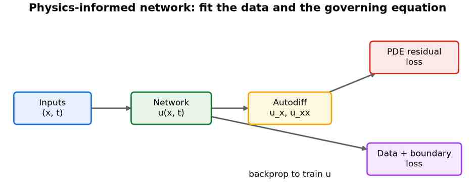
Origins and rise

Raissi, Perdikaris & Karniadakis introduced PINNs for both forward and inverse PDE problems.^[325] Operator-learning methods generalise further: DeepONet learns mappings between whole function spaces,^[326] and the Fourier Neural Operator learns resolution-independent solution operators in the spectral domain.^[327] The continuous-depth view connects them to neural ODEs.

Classical PINNs and variants

The original physics-informed neural network (PINN) stays close to the diagram in Fig 26: a single network whose loss blends data fit with the differential-equation residual.^[325] fPINNs extend the same residual idea to fractional derivatives,^[328] hp-VPINNs recast the loss in variational form with domain decomposition for stiffer problems,^[329] and B-PINNs turn the PINN Bayesian, placing a prior over the network and returning calibrated uncertainty in the solution.

Operator-learning networks

Where a PINN solves one instance of a PDE, operator learning learns the mapping from coefficient or boundary function to solution, generalising across the whole family. DeepONet branched into a branch net (encoding the input function) and a trunk net (encoding the query point)^[326] while the Fourier Neural Operator (FNO) parameterised the kernel in frequency space with a global FFT, making it fast and resolution-invariant.^[327] The Graph Neural Operator generalises FNO to irregular meshes, and MP-PDE casts the operator as message passing on a mesh graph, linking the approach to graph networks.^[330]

SciML frameworks

Building PINNs and operator networks by hand is laborious, so the community shipped general-purpose solvers. NeuralPDE (part of the SciML Julia ecosystem) and DeepXDE provide high-level APIs for declaring equations, boundary conditions, and architectures, and then dispatching training across backends — turning scientific machine learning from a research exercise into an engineering workflow.

Applications

• Solving and inverting PDEs in fluids, heat, and electromagnetics.
• Fast surrogates for expensive simulations.
• Data assimilation from sparse sensors.

Strengths and limitations

Strengths	Limitations
Work with little or no labelled data.	Training can be stiff and slow to converge.
Obey known physical laws.	Struggle with sharp or turbulent solutions.
Mesh-free, continuous solutions.	Often retrained per problem (operators help).

25. Audio, Speech & Music Networks

Audio networks turn waveforms or spectrograms into text, or text into audio. The pipeline in Fig 27 encodes the signal, models temporal context, and decodes to the target — reusing convolutional, recurrent, and Transformer machinery specialised for the time-frequency structure of sound.

Origins and rise

WaveNet generated raw audio sample by sample with dilated causal convolutions — the same structure as the TCN.^[87] Tacotron 2 synthesised natural speech by predicting mel-spectrograms and then vocoding them.^[331] For recognition, the Conformer fused convolution with self-attention,^[332] and Whisper reached robust multilingual transcription by training on very large weakly-labelled datasets.^[333]

Speech recognition

End-to-end networks replaced hand-engineered pipelines for converting speech to text. Deep Speech 2 used a deep recurrent or convolutional stack trained with CTC to map spectrograms to characters,^[334] the Jasper / QuartzNet family distilled the recipe into compact streaming convolutional architectures, and the Conformer interleaved convolutions with Transformer self-attention to capture both local and long-range acoustic cues.^[332] Whisper scaled weak supervision on 680 000 hours of web audio to a multilingual model that transcribes and translates without task-specific tuning.^[333]

Speech synthesis

On the generation side, Tacotron introduced attention-based end-to-end text-to-spectrogram synthesis^[331] and FastSpeech replaced the fragile autoregressive attention with a feed-forward Transformer that predicts mel-spectrogram durations in parallel,^[335] enabling fast and controllable synthesis. Neural vocoders such as WaveNet and HiFi-GAN then turn the spectrogram into audible waveform.

Music generation and source separation

Music raises longer-range structure than speech. The Music Transformer adapted relative self-attention to capture motifs and repetitions over thousands of notes,^[336] while MuseGAN took a GAN-based approach to multi-track symbolic generation. For separating instruments from a mixture, Conv-TasNet operates directly on the waveform with a learned encoder-decoder and masking network,^[337] and Demucs extends the idea to high-fidelity music separation with a U-Net-style structure.

Applications

• Speech recognition and text-to-speech synthesis.
• Music generation and source separation.
• Speaker verification and audio understanding.

Strengths and limitations

Strengths	Limitations
State-of-the-art speech and audio quality.	Heavy compute at high sample rates.
Reuse proven backbones.	Sensitive to noise and domain shift.
Scale with weakly-labelled data.	Real-time synthesis needs careful engineering.

26. Optical, Analog & Unconventional Networks

Not every neural network runs on a digital processor. Unconventional hardware performs the computation physically: a diffractive optical network, in Fig 28, sends light through a stack of passive, patterned layers whose interference implements the “weights,” and detectors read out the answer — inference at the speed of light with almost no power draw.

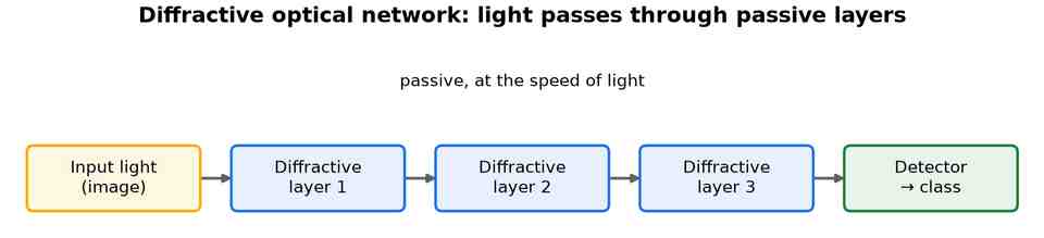
Origins and rise

Lin et al. built an all-optical diffractive deep neural network that classifies images passively.^[338] Shen et al. demonstrated a programmable nanophotonic processor performing matrix multiplication with interferometers.^[339] Related analog approaches use in-memory crossbar arrays and physical reservoirs, echoing the energy-efficiency goals of spiking networks.

Optical and photonic networks

Light computes convolutions at the speed of propagation. The diffractive deep neural network (D²NN) lays out successive diffractive optical layers and trains their phase masks so that the transmitted light pattern performs inference at the speed of light.^[338] Integrated photonic circuits carry the same idea onto a chip, using Mach-Zehnder interferometer meshes to perform matrix multiplication optically for low-energy inference.^[339]

Analog in-memory computing

Memristive crossbar arrays store weights as conductance levels and perform matrix-vector multiplication in a single analogue step by Kirchhoff's laws, making them natural for neuromorphic and edge inference. The trade-off is limited precision, device variability, and the difficulty of on-chip training, which is why most analogue arrays ship as accelerators for a frozen digital model.

Physical reservoir computing

A reservoir — any high-dimensional dynamical system — can serve as a fixed random feature map, leaving only a linear readout to be trained. Beyond the echo-state networks already discussed, researchers have built reservoirs from optical cavities, mechanical oscillators, and spintronic devices, exploiting their natural dynamics to classify temporal signals with minimal training energy.

Applications

• Ultra-low-power, low-latency inference.
• Optical front-ends for imaging and sensing.
• Edge accelerators for fixed models.

Strengths and limitations

Strengths	Limitations
Extremely fast, energy-efficient inference.	Fabrication fixes the weights; hard to retrain.
Massively parallel by physics.	Analog noise and calibration drift.
No digital multiply-accumulate.	Limited to specific, mostly linear operations.

27. Domain-Specific Architectures

Some of the largest breakthroughs are architectures tailored to a single domain. AlphaFold, in Fig 29, predicts protein structure by turning a sequence and its evolutionary relatives into pair features, refining them with attention (the Evoformer), and reading out 3-D atom coordinates — an accuracy leap on a decades-old problem.

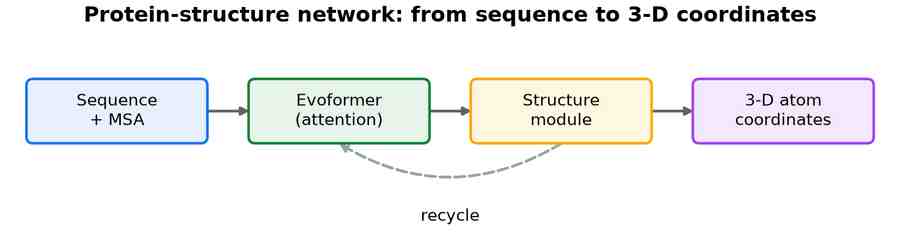
Origins and rise

AlphaFold combined attention over residues and residue pairs with a structure module and iterative recycling.^[340] In other domains, TabNet brought attention-based feature selection to tabular data,^[341] and vision-language-action models such as RT-2 repurposed multimodal Transformers as robot policies.^[342]

Tabular deep learning

TabNet brought sequential attention to tabular data, selecting features per example for both accuracy and interpretability^[341] while NODE generalised gradient-boosted trees into an end-to-end differentiable ensemble. The FT-Transformer and SAINT lines show that Transformer-style attention over columns, with intersample attention, can rival or beat gradient boosting on mid-sized tables.

Code generation

Programming languages are sequences too. CodeBERT extended masked-language pre-training to the bimodal code-and-text setting, and CodeT5 cast code understanding and generation into a unified text-to-text framework.^[343] AlphaCode scaled the same Transformer backbone with massive search and filtering to solve unseen competitive-programming problems, pointing toward systems that write software from a natural-language specification.

Protein and molecular structure

Perhaps the highest-impact domain-specific architecture is AlphaFold 2, whose Evoformer exchanges information across pair and multiple-sequence-alignment representations to predict 3D protein structure at experimental accuracy.^[340] RoseTTAFold offered a three-track alternative, and the ESM and ProtBERT protein language models bring the masked-pretraining recipe from natural language to amino-acid sequences, learning structure and function without labels.

Robotics and control

Robotics policies increasingly use large Transformer backbones. RT-1 showed that a vision-language-action Transformer can map camera input and natural-language commands to robot actions, and RT-2 demonstrated that co-fine-tuning a VLM on web-scale vision-language data and robot trajectories yields emergent semantic generalisation on the robot.^[342] SayCan grounds a language model's proposals in affordances learned from the robot itself, chaining skills into long-horizon plans.

Applications

• Protein-structure and molecular modelling.
• Tabular prediction in finance and healthcare.
• Language-conditioned robotic control.

Strengths and limitations

Strengths	Limitations
Superhuman accuracy within their niche.	Narrow, with heavy domain engineering.
Encode domain priors directly.	Need large, curated datasets.
Reuse attention and multimodal ideas.	Expensive to train and adapt.

28. Combined & Hybrid Architectures

Finally, many production systems are hybrids that chain families end to end. A classic pattern, in Fig 30, feeds convolutional features into a recurrent model: a CNN reads the image or video frames, and an RNN turns the resulting feature sequence into text — the recipe behind OCR and video captioning.

Origins and rise

The CRNN combined convolution, recurrence, and a sequence loss for image-based text recognition.^[344] As models scaled, mixture-of-experts hybrids such as the Switch Transformer routed each token to a subset of expert sub-networks, growing capacity without a proportional rise in compute.^[57] Other common hybrids marry CNNs with Transformers, or attention with recurrent sequence-to-sequence models.

CNN + RNN hybrids

Marrying a convolutional feature extractor with a recurrent head was the dominant recipe for video and sequence tasks before Transformers. A CNN-LSTM feeds per-frame CNN features into an LSTM for video captioning or action recognition, and CRNN (a CNN+RNN+CTC pipeline) became the standard architecture for optical character recognition, reading text as a sequence of image columns.

CNN + Transformer hybrids

Vision models increasingly blend the locality and translation invariance of convolution with the global context of self-attention. ConViT initialised a Vision Transformer with convolutional soft inductive biases, LeViT traded classification accuracy for fast inference by interleaving conv and attention stages, and MobileViT fused the mobile-CNN block design with Transformer blocks for lightweight mobile vision.

RNN + Attention (sequence-to-sequence)

The original attention mechanism was itself a hybrid: Bahdanau attention added a learned alignment between an encoder RNN and a decoder RNN, letting the decoder look back at all source hidden states for each output word.^[345] Luong attention simplified and generalised the scoring, and this encoder-decoder-plus-attention recipe dominated machine translation until the fully-attentional Transformer replaced the recurrent backbone.

Mixture-of-experts and ensembles

Scaling width is expensive, so mixture-of-experts (MoE) models sparsely activate a few expert sub-networks per token via a learned gating function. The Switch Transformer routed to a single expert per token to scale to trillions of parameters,^[57] GLaM and DeepSpeed-MoE refined the routing and load-balancing, and Mixtral brought sparse MoE into the open-weight LLM mainstream. Ensembles such as the basis-mixing in N-BEATS take a different route to the same goal: combine many diverse models into one robust forecast.

Applications

• Optical character recognition and video captioning.
• Scalable large language models via sparse experts.
• Any task where one family's output is another's input.

Strengths and limitations

Strengths	Limitations
Combine complementary strengths.	More moving parts to train and tune.
Reuse proven components.	Interfaces between modules add complexity.
Scale capacity, e.g. via mixture of experts.	Harder to debug and deploy.

Key takeaways

• A neural network is a stack of simple weighted units trained by backpropagation; every family here is that idea plus structure suited to a kind of data.
• Feedforward networks are the universal baseline and the output head of almost everything else.
• Convolutional networks add weight sharing for images; residual connections made them very deep.
• Recurrent networks handle sequences with a running state, and gates gave them longer memory.
• The Transformer swapped recurrence for attention, unlocking parallel training and today's large models across every modality.
• Generative models reuse those same backbones to sample new data rather than label it.
• Beyond these backbones, specialised families adapt the same machinery to other data and goals — graphs, spikes, and multiple modalities — while paradigms such as reinforcement learning and architecture search change how networks are trained and designed.
• The long tail specialises further still — recommenders, point clouds, time series, physics-informed solvers, and domain-specific models like AlphaFold — and the most capable systems are often hybrids that chain several families end to end.

Resources

The sources below are numbered in order of first appearance in the text; each bracketed marker such as ^[1] links to its entry. Entries are the seminal papers and datasets behind each family; the diagrams in this article are original schematics drawn for it, not reproductions of any third-party figure.

• [1] Deep Learning — LeCun, Bengio & Hinton, Nature, 2015. nature.com
• [2] A Logical Calculus of the Ideas Immanent in Nervous Activity — McCulloch & Pitts, Bulletin of Mathematical Biophysics, 1943. springer.com
• [3] The Perceptron: A Probabilistic Model — Rosenblatt, Psychological Review, 1958. apa.org
• [4] Learning Representations by Back-propagating Errors — Rumelhart, Hinton & Williams, Nature, 1986. nature.com
• [5] Multilayer Feedforward Networks are Universal Approximators — Hornik, Stinchcombe & White, Neural Networks, 1989. doi.org
• [6] Reducing the Dimensionality of Data with Neural Networks — Hinton & Salakhutdinov, Science, 2006. doi.org
• [7] A Fast Learning Algorithm for Deep Belief Nets — Hinton, Osindero & Teh, Neural Computation, 2006. doi.org
• [8] Extreme Learning Machine: Theory and Applications — Huang, Zhu & Siew, Neurocomputing, 2006. doi.org
• [9] Neocognitron: A Self-Organizing Neural Network Model for a Mechanism of Pattern Recognition Unaffected by Shift in Position — Fukushima, Biological Cybernetics, 1980. doi.org
• [10] Gradient-Based Learning Applied to Document Recognition (LeNet-5) — LeCun, Bottou, Bengio & Haffner, Proc. IEEE, 1998. lecun.com
• [11] ImageNet Classification with Deep Convolutional Neural Networks (AlexNet) — Krizhevsky, Sutskever & Hinton, NeurIPS, 2012. papers.nips.cc
• [12] ImageNet: A Large-Scale Hierarchical Image Database — Deng et al., CVPR, 2009. Dataset, custom research license. image-net.org
• [13] Very Deep Convolutional Networks for Large-Scale Image Recognition (VGG) — Simonyan & Zisserman, ICLR, 2015. arxiv.org/abs/1409.1556
• [14] Deep Residual Learning for Image Recognition (ResNet) — He, Zhang, Ren & Sun, CVPR, 2016. arxiv.org/abs/1512.03385
• [15] Going Deeper with Convolutions (GoogLeNet / Inception) — Szegedy et al., CVPR, 2015. arxiv.org/abs/1409.4842
• [16] Densely Connected Convolutional Networks (DenseNet) — Huang, Liu, van der Maaten & Weinberger, CVPR, 2017. arxiv.org/abs/1608.06993
• [17] MobileNets: Efficient Convolutional Neural Networks for Mobile Vision Applications — Howard et al., 2017. arxiv.org/abs/1704.04861
• [18] EfficientNet: Rethinking Model Scaling for Convolutional Neural Networks — Tan & Le, ICML, 2019. arxiv.org/abs/1905.11946
• [19] A ConvNet for the 2020s (ConvNeXt) — Liu et al., CVPR, 2022. arxiv.org/abs/2201.03545
• [20] Faster R-CNN: Towards Real-Time Object Detection with Region Proposal Networks — Ren, He, Girshick & Sun, NeurIPS, 2015. arxiv.org/abs/1506.01497
• [21] You Only Look Once: Unified, Real-Time Object Detection (YOLO) — Redmon, Divvala, Girshick & Farhadi, CVPR, 2016. arxiv.org/abs/1506.02640
• [22] Focal Loss for Dense Object Detection (RetinaNet) — Lin et al., ICCV, 2017. arxiv.org/abs/1708.02002
• [23] End-to-End Object Detection with Transformers (DETR) — Carion et al., ECCV, 2020. arxiv.org/abs/2005.12872
• [24] Fully Convolutional Networks for Semantic Segmentation — Long, Shelhamer & Darrell, CVPR, 2015. arxiv.org/abs/1411.4038
• [25] U-Net: Convolutional Networks for Biomedical Image Segmentation — Ronneberger, Fischer & Brox, MICCAI, 2015. arxiv.org/abs/1505.04597
• [26] Rethinking Atrous Convolution for Semantic Image Segmentation (DeepLabv3) — Chen, Papandreou, Schroff & Adam, 2017. arxiv.org/abs/1706.05587
• [27] Mask R-CNN — He, Gkioxari, Dollár & Girshick, ICCV, 2017. arxiv.org/abs/1703.06870
• [28] Segment Anything (SAM) — Kirillov et al., ICCV, 2023. arxiv.org/abs/2304.02643
• [29] Quo Vadis, Action Recognition? A New Model and the Kinetics Dataset (I3D) — Carreira & Zisserman, CVPR, 2017. arxiv.org/abs/1705.07750
• [30] SlowFast Networks for Video Recognition — Feichtenhofer, Fan, Malik & He, ICCV, 2019. arxiv.org/abs/1812.03982
• [31] Image Super-Resolution Using Deep Convolutional Networks (SRCNN) — Dong, Loy, He & Tang, IEEE TPAMI, 2016. arxiv.org/abs/1501.00092
• [32] ESRGAN: Enhanced Super-Resolution Generative Adversarial Networks — Wang et al., ECCV Workshops, 2018. arxiv.org/abs/1809.00219
• [33] SwinIR: Image Restoration Using Swin Transformer — Liang et al., ICCV Workshops, 2021. arxiv.org/abs/2108.10257
• [34] Finding Structure in Time — Elman, Cognitive Science, 1990. doi.org
• [35] Long Short-Term Memory (LSTM) — Hochreiter & Schmidhuber, Neural Computation, 1997. doi.org
• [36] Learning Phrase Representations using RNN Encoder-Decoder (GRU) — Cho et al., EMNLP, 2014. arxiv.org/abs/1406.1078
• [37] Bidirectional Recurrent Neural Networks — Schuster & Paliwal, IEEE Transactions on Signal Processing, 1997. doi.org
• [38] Convolutional LSTM Network: A Machine Learning Approach for Precipitation Nowcasting — Shi et al., NeurIPS, 2015. arxiv.org/abs/1506.04214
• [39] Quasi-Recurrent Neural Networks — Bradbury, Merity, Xiong & Socher, ICLR, 2017. arxiv.org/abs/1611.01576
• [40] Simple Recurrent Units for Highly Parallelizable Recurrence — Lei et al., EMNLP, 2018. arxiv.org/abs/1709.02755
• [41] Independently Recurrent Neural Network (IndRNN): Building A Longer and Deeper RNN — Li et al., CVPR, 2018. arxiv.org/abs/1803.04831
• [42] Neural Turing Machines — Graves, Wayne & Danihelka, 2014. arxiv.org/abs/1410.5401
• [43] Hybrid Computing Using a Neural Network with Dynamic External Memory (DNC) — Graves et al., Nature, 2016. nature.com
• [44] End-To-End Memory Networks — Sukhbaatar, Szlam, Weston & Fergus, NeurIPS, 2015. arxiv.org/abs/1503.08895
• [45] Harnessing Nonlinearity: Predicting Chaotic Systems and Saving Energy in Wireless Communication (Echo State Network) — Jaeger & Haas, Science, 2004. doi.org
• [46] Real-Time Computing Without Stable States: A New Framework for Neural Computation Based on Perturbations (Liquid State Machine) — Maass, Natschläger & Markram, Neural Computation, 2002. doi.org
• [47] Attention Is All You Need — Vaswani et al., NeurIPS, 2017. arxiv.org/abs/1706.03762
• [48] BERT: Pre-training of Deep Bidirectional Transformers — Devlin et al., NAACL, 2019. arxiv.org/abs/1810.04805
• [49] Language Models are Few-Shot Learners (GPT-3) — Brown et al., NeurIPS, 2020. arxiv.org/abs/2005.14165
• [50] An Image is Worth 16×16 Words (Vision Transformer) — Dosovitskiy et al., ICLR, 2021. arxiv.org/abs/2010.11929
• [51] RoBERTa: A Robustly Optimized BERT Pretraining Approach — Liu et al., 2019. arxiv.org/abs/1907.11692
• [52] ELECTRA: Pre-training Text Encoders as Discriminators Rather Than Generators — Clark et al., ICLR, 2020. arxiv.org/abs/2003.10555
• [53] DeBERTa: Decoding-enhanced BERT with Disentangled Attention — He et al., ICLR, 2021. arxiv.org/abs/2006.03654
• [54] Training Compute-Optimal Large Language Models (Chinchilla) — Hoffmann et al., NeurIPS, 2022. arxiv.org/abs/2203.15556
• [55] PaLM: Scaling Language Modeling with Pathways — Chowdhery et al., JMLR, 2023. arxiv.org/abs/2204.02311
• [56] LLaMA: Open and Efficient Foundation Language Models — Touvron et al., 2023. arxiv.org/abs/2302.13971
• [57] Switch Transformers: Scaling to Trillion Parameter Models with Simple and Efficient Sparsity — Fedus, Zoph & Shazeer, JMLR, 2022. arxiv.org/abs/2101.03961
• [58] Exploring the Limits of Transfer Learning with a Unified Text-to-Text Transformer (T5) — Raffel et al., JMLR, 2020. arxiv.org/abs/1910.10683
• [59] BART: Denoising Sequence-to-Sequence Pre-training — Lewis et al., ACL, 2020. arxiv.org/abs/1910.13461
• [60] Training Data-Efficient Image Transformers & Distillation through Attention (DeiT) — Touvron et al., ICML, 2021. arxiv.org/abs/2012.12877
• [61] Swin Transformer: Hierarchical Vision Transformer using Shifted Windows — Liu et al., ICCV, 2021. arxiv.org/abs/2103.14030
• [62] BEiT: BERT Pre-Training of Image Transformers — Bao et al., ICLR, 2022. arxiv.org/abs/2106.08254
• [63] Masked Autoencoders Are Scalable Vision Learners — He et al., CVPR, 2022. arxiv.org/abs/2111.06377
• [64] Emerging Properties in Self-Supervised Vision Transformers (DINO) — Caron et al., ICCV, 2021. arxiv.org/abs/2104.14294
• [65] Longformer: The Long-Document Transformer — Beltagy et al., 2020. arxiv.org/abs/2004.05150
• [66] Big Bird: Transformers for Longer Sequences — Zaheer et al., NeurIPS, 2020. arxiv.org/abs/2007.14062
• [67] Reformer: The Efficient Transformer — Kitaev et al., ICLR, 2020. arxiv.org/abs/2001.04451
• [68] Rethinking Attention with Performers — Choromanski et al., ICLR, 2021. arxiv.org/abs/2009.14794
• [69] FlashAttention: Fast and Memory-Efficient Exact Attention with IO-Awareness — Dao et al., NeurIPS, 2022. arxiv.org/abs/2205.14135
• [70] Decision Transformer: Reinforcement Learning via Sequence Modeling — Chen et al., NeurIPS, 2021. arxiv.org/abs/2106.01345
• [71] A Generalist Agent (Gato) — Reed et al., TMLR, 2022. arxiv.org/abs/2205.06175
• [72] Generative Adversarial Nets (GAN) — Goodfellow et al., NeurIPS, 2014. arxiv.org/abs/1406.2661
• [73] Auto-Encoding Variational Bayes (VAE) — Kingma & Welling, ICLR, 2014. arxiv.org/abs/1312.6114
• [74] Denoising Diffusion Probabilistic Models (DDPM) — Ho, Jain & Abbeel, NeurIPS, 2020. arxiv.org/abs/2006.11239
• [75] High-Resolution Image Synthesis with Latent Diffusion Models (Stable Diffusion) — Rombach et al., CVPR, 2022. arxiv.org/abs/2112.10752
• [76] Unsupervised Representation Learning with Deep Convolutional GANs (DCGAN) — Radford, Metz & Chintala, ICLR, 2016. arxiv.org/abs/1511.06434
• [77] Wasserstein GAN — Arjovsky, Chintala & Bottou, ICML, 2017. arxiv.org/abs/1701.07875
• [78] Self-Attention Generative Adversarial Networks (SAGAN) — Zhang et al., ICML, 2019. arxiv.org/abs/1805.08318
• [79] Progressive Growing of GANs for Improved Quality, Stability, and Variation — Karras et al., ICLR, 2018. arxiv.org/abs/1710.10196
• [80] A Style-Based Generator Architecture for GANs (StyleGAN) — Karras, Laine & Aila, CVPR, 2019. arxiv.org/abs/1812.04948
• [81] Large Scale GAN Training for High Fidelity Natural Image Synthesis (BigGAN) — Brock, Donahue & Simonyan, ICLR, 2019. arxiv.org/abs/1809.11096
• [82] Image-to-Image Translation with Conditional Adversarial Networks (Pix2Pix) — Isola et al., CVPR, 2017. arxiv.org/abs/1611.07004
• [83] Unpaired Image-to-Image Translation using Cycle-Consistent Adversarial Networks (CycleGAN) — Zhu et al., ICCV, 2017. arxiv.org/abs/1703.10593
• [84] Neural Discrete Representation Learning (VQ-VAE) — van den Oord, Vinyals & Kavukcuoglu, NeurIPS, 2017. arxiv.org/abs/1711.00937
• [85] Taming Transformers for High-Resolution Image Synthesis (VQGAN) — Esser, Rombach & Ommer, CVPR, 2021. arxiv.org/abs/2012.09841
• [86] Pixel Recurrent Neural Networks — van den Oord, Kalchbrenner & Kavukcuoglu, ICML, 2016. arxiv.org/abs/1601.06759
• [87] WaveNet: A Generative Model for Raw Audio — van den Oord et al., 2016. arxiv.org/abs/1609.03499
• [88] Denoising Diffusion Implicit Models (DDIM) — Song, Meng & Ermon, ICLR, 2021. arxiv.org/abs/2010.02502
• [89] Score-Based Generative Modeling through Stochastic Differential Equations — Song et al., ICLR, 2021. arxiv.org/abs/2011.13456
• [90] Diffusion Models Beat GANs on Image Synthesis — Dhariwal & Nichol, NeurIPS, 2021. arxiv.org/abs/2105.05233
• [91] SDXL: Improving Latent Diffusion Models for High-Resolution Image Synthesis — Podell et al., 2023. arxiv.org/abs/2307.01952
• [92] DPM-Solver: A Fast ODE Solver for Diffusion Probabilistic Model Sampling — Lu et al., NeurIPS, 2022. arxiv.org/abs/2206.00927
• [93] Density Estimation using Real NVP — Dinh, Sohl-Dickstein & Bengio, ICLR, 2017. arxiv.org/abs/1605.08803
• [94] Glow: Generative Flow with Invertible 1×1 Convolutions — Kingma & Dhariwal, NeurIPS, 2018. arxiv.org/abs/1807.03039
• [95] Your Classifier is Secretly an Energy Based Model (JEM) — Grathwohl et al., ICLR, 2020. arxiv.org/abs/1912.03263
• [96] Semi-Supervised Classification with Graph Convolutional Networks (GCN) — Kipf & Welling, ICLR, 2017. arxiv.org/abs/1609.02907
• [97] Graph Attention Networks (GAT) — Veličković et al., ICLR, 2018. arxiv.org/abs/1710.10903
• [98] Convolutional Neural Networks on Graphs with Fast Localized Spectral Filtering (ChebNet) — Defferrard, Bresson & Vandergheynst, NeurIPS, 2016. arxiv.org/abs/1606.09375
• [99] Inductive Representation Learning on Large Graphs (GraphSAGE) — Hamilton, Ying & Leskovec, NeurIPS, 2017. arxiv.org/abs/1706.02216
• [100] Neural Message Passing for Quantum Chemistry (MPNN) — Gilmer et al., ICML, 2017. arxiv.org/abs/1704.01212
• [101] How Powerful are Graph Neural Networks? (GIN) — Xu et al., ICLR, 2019. arxiv.org/abs/1810.00826
• [102] SchNet: A Continuous-Filter Convolutional Neural Network for Modeling Quantum Interactions — Schütt et al., NeurIPS, 2017. arxiv.org/abs/1706.08566
• [103] SE(3)-Transformers: 3D Roto-Translation Equivariant Attention Networks — Fuchs et al., NeurIPS, 2020. arxiv.org/abs/2006.10503
• [104] Spatial Temporal Graph Convolutional Networks for Skeleton-Based Action Recognition (ST-GCN) — Yan, Xiong & Lin, AAAI, 2018. arxiv.org/abs/1801.07455
• [105] Graph WaveNet for Deep Spatial-Temporal Graph Modeling — Wu et al., IJCAI, 2019. arxiv.org/abs/1906.00121
• [106] Do Transformers Really Perform Bad for Graph Representation? (Graphormer) — Ying et al., NeurIPS, 2021. arxiv.org/abs/2106.05234
• [107] Graph Contrastive Learning with Augmentations (GraphCL) — You et al., NeurIPS, 2020. arxiv.org/abs/2010.13902
• [108] Self-Organized Formation of Topologically Correct Feature Maps — Kohonen, Biological Cybernetics, 1982. doi.org
• [109] The Growing Hierarchical Self-Organizing Map: Exploratory Analysis of High-Dimensional Data — Rauber, Merkl & Dittenbach, IEEE Transactions on Neural Networks, 2002. doi.org
• [110] ‘Neural-Gas’ Network for Vector Quantization and its Application to Time-Series Prediction — Martinetz, Berkovich & Schulten, IEEE Transactions on Neural Networks, 1993. doi.org
• [111] A Self-Organising Network that Grows When Required (GWR) — Marsland, Shapiro & Nehmzow, Neural Networks, 2002. doi.org
• [112] A Review of Learning Vector Quantization Classifiers — Nova & Estévez, Neural Computing and Applications, 2014. doi.org
• [113] Dynamic Routing Between Capsules — Sabour, Frosst & Hinton, NeurIPS, 2017. arxiv.org/abs/1710.09829
• [114] Matrix Capsules with EM Routing — Hinton, Sabour & Frosst, ICLR, 2018. openreview.net
• [115] DeepCaps: Going Deeper with Capsule Networks — Rajasegaran et al., CVPR, 2019. arxiv.org/abs/1904.09546
• [116] Stacked Capsule Autoencoders — Kosiorek, Sabour, Teh & Hinton, NeurIPS, 2019. arxiv.org/abs/1906.06818
• [117] 3D Point Capsule Networks — Zhao, Birdal, Deng & Tombari, CVPR, 2019. arxiv.org/abs/1812.10775
• [118] Signature Verification using a Siamese Time Delay Neural Network — Bromley et al., NeurIPS, 1993. papers.nips.cc
• [119] FaceNet: A Unified Embedding for Face Recognition and Clustering — Schroff, Kalenichenko & Philbin, CVPR, 2015. arxiv.org/abs/1503.03832
• [120] Dimensionality Reduction by Learning an Invariant Mapping (Contrastive Loss) — Hadsell, Chopra & LeCun, CVPR, 2006. doi.org
• [121] Deep Metric Learning via Lifted Structured Feature Embedding — Song, Xiang, Jegelka & Savarese, CVPR, 2016. arxiv.org/abs/1511.06452
• [122] Matching Networks for One Shot Learning — Vinyals et al., NeurIPS, 2016. arxiv.org/abs/1606.04080
• [123] Prototypical Networks for Few-shot Learning — Snell, Swersky & Zemel, NeurIPS, 2017. arxiv.org/abs/1703.05175
• [124] Learning to Compare: Relation Network for Few-Shot Learning — Sung et al., CVPR, 2018. arxiv.org/abs/1711.06025
• [125] A Simple Framework for Contrastive Learning of Visual Representations (SimCLR) — Chen, Kornblith, Norouzi & Hinton, ICML, 2020. arxiv.org/abs/2002.05709
• [126] Momentum Contrast for Unsupervised Visual Representation Learning (MoCo) — He, Fan, Wu, Xie & Girshick, CVPR, 2020. arxiv.org/abs/1911.05722
• [127] Bootstrap Your Own Latent: A New Approach to Self-Supervised Learning (BYOL) — Grill et al., NeurIPS, 2020. arxiv.org/abs/2006.07733
• [128] Exploring Simple Siamese Representation Learning (SimSiam) — Chen & He, CVPR, 2021. arxiv.org/abs/2011.10566
• [129] Unsupervised Learning of Visual Features by Contrasting Cluster Assignments (SwAV) — Caron et al., NeurIPS, 2020. arxiv.org/abs/2006.09882
• [130] Barlow Twins: Self-Supervised Learning via Redundancy Reduction — Zbontar, Jing, Misra, LeCun & Deny, ICML, 2021. arxiv.org/abs/2103.03230
• [131] VICReg: Variance-Invariance-Covariance Regularization for Self-Supervised Learning — Bardes, Ponce & LeCun, ICLR, 2022. arxiv.org/abs/2105.04906
• [132] ArcFace: Additive Angular Margin Loss for Deep Face Recognition — Deng, Guo, Yang, Xue, Kotsia & Zafeiriou, CVPR, 2019. arxiv.org/abs/1801.07698
• [133] Proxy Anchor Loss for Deep Metric Learning — Kim, Kim, Cho & Kwak, CVPR, 2020. arxiv.org/abs/2003.13911
• [134] Multi-Similarity Loss with General Pair Weighting for Deep Metric Learning — Wang, Han, Huang, Dong & Scott, CVPR, 2019. arxiv.org/abs/1904.06627
• [135] Circle Loss: A Unified Perspective of Pair Similarity Optimization — Sun et al., CVPR, 2020. arxiv.org/abs/2002.10857
• [136] Neural Ordinary Differential Equations — Chen, Rubanova, Bettencourt & Duvenaud, NeurIPS, 2018. arxiv.org/abs/1806.07366
• [137] Augmented Neural ODEs — Dupont, Doucet & Teh, NeurIPS, 2019. arxiv.org/abs/1904.01681
• [138] Latent ODEs for Irregularly-Sampled Time Series — Rubanova, Chen & Duvenaud, NeurIPS, 2019. arxiv.org/abs/1907.03907
• [139] Neural Controlled Differential Equations for Irregular Time Series — Kidger, Morrill, Foster & Lyons, NeurIPS, 2020. arxiv.org/abs/2005.08926
• [140] FFJORD: Free-form Continuous Dynamics for Scalable Reversible Generative Models — Grathwohl, Chen, Bettencourt, Sutskever & Duvenaud, ICLR, 2019. arxiv.org/abs/1810.01367
• [141] Scalable Gradients for Stochastic Differential Equations — Li, Wong, Chen & Duvenaud, AISTATS, 2020. arxiv.org/abs/2001.01328
• [142] Neural SDEs as Infinite-Dimensional GANs — Kidger, Foster, Li, Oberhauser & Lyons, ICML, 2021. arxiv.org/abs/2102.03657
• [143] Networks of Spiking Neurons: The Third Generation of Neural Network Models — Maass, Neural Networks, 1997. doi.org
• [144] Surrogate Gradient Learning in Spiking Neural Networks — Neftci, Mostafa & Zenke, IEEE Signal Processing Magazine, 2019. arxiv.org/abs/1901.09948
• [145] Simple Model of Spiking Neurons — Izhikevich, IEEE Transactions on Neural Networks, 2003. doi.org
• [146] Adaptive Exponential Integrate-and-Fire Model as an Effective Description of Neuronal Activity (AdEx) — Brette & Gerstner, Journal of Neurophysiology, 2005. doi.org
• [147] Unsupervised Learning of Digit Recognition Using Spike-Timing-Dependent Plasticity — Diehl & Cook, Frontiers in Computational Neuroscience, 2015. doi.org
• [148] Conversion of Continuous-Valued Deep Networks to Efficient Event-Driven Networks for Image Classification — Rueckauer et al., Frontiers in Neuroscience, 2017. doi.org
• [149] Going Deeper in Spiking Neural Networks: VGG and Residual Architectures — Sengupta et al., Frontiers in Neuroscience, 2019. arxiv.org/abs/1802.02627
• [150] SLAYER: Spike Layer Error Reassignment in Time — Shrestha & Orchard, NeurIPS, 2018. arxiv.org/abs/1810.08646
• [151] Going Deeper With Directly-Trained Larger Spiking Neural Networks — Zheng et al., AAAI, 2021. arxiv.org/abs/2011.05280
• [152] Spikformer: When Spiking Neural Network Meets Transformer — Zhou et al., ICLR, 2023. arxiv.org/abs/2209.15425
• [153] Long Short-Term Memory and Learning-to-Learn in Networks of Spiking Neurons (LSNN) — Bellec et al., NeurIPS, 2018. arxiv.org/abs/1803.09574
• [154] A Million Spiking-Neuron Integrated Circuit with a Scalable Communication Network and Interface (TrueNorth) — Merolla et al., Science, 2014. doi.org
• [155] Loihi: A Neuromorphic Manycore Processor with On-Chip Learning — Davies et al., IEEE Micro, 2018. doi.org
• [156] Squeeze-and-Excitation Networks (SENet) — Hu, Shen & Sun, CVPR, 2018. arxiv.org/abs/1709.01507
• [157] CBAM: Convolutional Block Attention Module — Woo et al., ECCV, 2018. arxiv.org/abs/1807.06521
• [158] ECA-Net: Efficient Channel Attention for Deep Convolutional Neural Networks — Wang et al., CVPR, 2020. arxiv.org/abs/1910.03151
• [159] Selective Kernel Networks (SKNet) — Li et al., CVPR, 2019. arxiv.org/abs/1903.06586
• [160] BAM: Bottleneck Attention Module — Park et al., BMVC, 2018. arxiv.org/abs/1807.06514
• [161] Non-local Neural Networks — Wang, Girshick, Gupta & He, CVPR, 2018. arxiv.org/abs/1711.07971
• [162] GCNet: Non-local Networks Meet Squeeze-Excitation Networks and Beyond — Cao et al., ICCV Workshops, 2019. arxiv.org/abs/1904.11492
• [163] CCNet: Criss-Cross Attention for Semantic Segmentation — Huang et al., ICCV, 2019. arxiv.org/abs/1811.11721
• [164] Stand-Alone Self-Attention in Vision Models — Ramachandran et al., NeurIPS, 2019. arxiv.org/abs/1906.05909
• [165] Axial-DeepLab: Stand-Alone Axial-Attention for Panoptic Segmentation — Wang et al., ECCV, 2020. arxiv.org/abs/2003.07853
• [166] Neural Architecture Search with Reinforcement Learning — Zoph & Le, ICLR, 2017. arxiv.org/abs/1611.01578
• [167] DARTS: Differentiable Architecture Search — Liu, Simonyan & Yang, ICLR, 2019. arxiv.org/abs/1806.09055
• [168] Learning Transferable Architectures for Scalable Image Recognition (NASNet) — Zoph, Vasudevan, Shlens & Le, CVPR, 2018. arxiv.org/abs/1707.07012
• [169] Efficient Neural Architecture Search via Parameter Sharing (ENAS) — Pham et al., ICML, 2018. arxiv.org/abs/1802.03268
• [170] PC-DARTS: Partial Channel Connections for Memory-Efficient Architecture Search — Xu et al., ICLR, 2020. arxiv.org/abs/1907.05737
• [171] Progressive Differentiable Architecture Search: Bridging the Depth Gap between Search and Evaluation (P-DARTS) — Chen et al., ICCV, 2019. arxiv.org/abs/1904.12760
• [172] Fair DARTS: Eliminating Unfair Advantages in Differentiable Architecture Search — Chu et al., ECCV, 2020. arxiv.org/abs/1911.12126
• [173] DARTS-: Robustly Stepping out of Performance Collapse Without Indicators — Chu et al., ICLR, 2021. arxiv.org/abs/2009.01027
• [174] MnasNet: Platform-Aware Neural Architecture Search for Mobile — Tan et al., CVPR, 2019. arxiv.org/abs/1807.11626
• [175] MixConv: Mixed Depthwise Convolutional Kernels (MixNet) — Tan & Le, BMVC, 2019. arxiv.org/abs/1907.09595
• [176] ProxylessNAS: Direct Neural Architecture Search on Target Task and Hardware — Cai, Zhu & Han, ICLR, 2019. arxiv.org/abs/1812.00332
• [177] FBNet: Hardware-Aware Efficient ConvNet Design via Differentiable Neural Architecture Search — Wu et al., CVPR, 2019. arxiv.org/abs/1812.03443
• [178] HAT: Hardware-Aware Transformers for Efficient Natural Language Processing — Wang et al., ACL, 2020. arxiv.org/abs/2005.14187
• [179] Once-for-All: Train One Network and Specialize it for Efficient Deployment — Cai et al., ICLR, 2020. arxiv.org/abs/1908.09791
• [180] BigNAS: Scaling Up Neural Architecture Search with Big Single-Stage Models — Yu et al., ECCV, 2020. arxiv.org/abs/2003.11142
• [181] SCARLET-NAS: Bridging the Gap between Stability and Scalability in Weight-sharing Neural Architecture Search — Chu et al., 2021. arxiv.org/abs/1908.06022
• [182] AutoFormer: Searching Transformers for Visual Recognition — Chen et al., ICCV, 2021. arxiv.org/abs/2107.00651
• [183] Designing Network Design Spaces (RegNet) — Radosavovic et al., CVPR, 2020. arxiv.org/abs/2003.13678
• [184] Human-Level Control through Deep Reinforcement Learning (DQN) — Mnih et al., Nature, 2015. nature.com
• [185] Proximal Policy Optimization Algorithms (PPO) — Schulman et al., 2017. arxiv.org/abs/1707.06347
• [186] Deep Reinforcement Learning with Double Q-learning (Double DQN) — van Hasselt, Guez & Silver, AAAI, 2016. arxiv.org/abs/1509.06461
• [187] Dueling Network Architectures for Deep Reinforcement Learning — Wang et al., ICML, 2016. arxiv.org/abs/1511.06581
• [188] A Distributional Perspective on Reinforcement Learning (C51) — Bellemare, Dabney & Munos, ICML, 2017. arxiv.org/abs/1707.06887
• [189] Distributional Reinforcement Learning with Quantile Regression (QR-DQN) — Dabney et al., AAAI, 2018. arxiv.org/abs/1710.10044
• [190] Implicit Quantile Networks for Distributional Reinforcement Learning (IQN) — Dabney et al., ICML, 2018. arxiv.org/abs/1806.06923
• [191] Rainbow: Combining Improvements in Deep Reinforcement Learning — Hessel et al., AAAI, 2018. arxiv.org/abs/1710.02298
• [192] Distributed Prioritized Experience Replay (Ape-X) — Horgan et al., ICLR, 2018. arxiv.org/abs/1803.00933
• [193] Asynchronous Methods for Deep Reinforcement Learning (A3C) — Mnih et al., ICML, 2016. arxiv.org/abs/1602.01783
• [194] Trust Region Policy Optimization (TRPO) — Schulman et al., ICML, 2015. arxiv.org/abs/1502.05477
• [195] Continuous Control with Deep Reinforcement Learning (DDPG) — Lillicrap et al., ICLR, 2016. arxiv.org/abs/1509.02971
• [196] Addressing Function Approximation Error in Actor-Critic Methods (TD3) — Fujimoto, van Hoof & Meger, ICML, 2018. arxiv.org/abs/1802.09477
• [197] Soft Actor-Critic: Off-Policy Maximum Entropy Deep Reinforcement Learning (SAC) — Haarnoja et al., ICML, 2018. arxiv.org/abs/1801.01290
• [198] World Models — Ha & Schmidhuber, NeurIPS, 2018. arxiv.org/abs/1803.10122
• [199] Learning Latent Dynamics for Planning from Pixels (PlaNet) — Hafner et al., ICML, 2019. arxiv.org/abs/1811.04551
• [200] Mastering Diverse Domains through World Models (DreamerV3) — Hafner et al., 2023. arxiv.org/abs/2301.04104
• [201] Mastering Atari, Go, Chess and Shogi by Planning with a Learned Model (MuZero) — Schrittwieser et al., Nature, 2020. arxiv.org/abs/1911.08265
• [202] Mastering Atari Games with Limited Data (EfficientZero) — Ye et al., NeurIPS, 2021. arxiv.org/abs/2111.00210
• [203] Multi-Agent Actor-Critic for Mixed Cooperative-Competitive Environments (MADDPG) — Lowe et al., NeurIPS, 2017. arxiv.org/abs/1706.02275
• [204] Value-Decomposition Networks for Cooperative Multi-Agent Learning (VDN) — Sunehag et al., AAMAS, 2018. arxiv.org/abs/1706.05296
• [205] QMIX: Monotonic Value Function Factorisation for Deep Multi-Agent Reinforcement Learning — Rashid et al., ICML, 2018. arxiv.org/abs/1803.11485
• [206] Counterfactual Multi-Agent Policy Gradients (COMA) — Foerster et al., AAAI, 2018. arxiv.org/abs/1705.08926
• [207] The Surprising Effectiveness of PPO in Cooperative, Multi-Agent Games (MAPPO) — Yu et al., NeurIPS, 2022. arxiv.org/abs/2103.01955
• [208] Learning Transferable Visual Models From Natural Language Supervision (CLIP) — Radford et al., ICML, 2021. arxiv.org/abs/2103.00020
• [209] Flamingo: a Visual Language Model for Few-Shot Learning — Alayrac et al., NeurIPS, 2022. arxiv.org/abs/2204.14198
• [210] Scaling Up Visual and Vision-Language Representation Learning With Noisy Text Supervision (ALIGN) — Jia et al., ICML, 2021. arxiv.org/abs/2102.05918
• [211] LiT: Zero-Shot Transfer with Locked-image Text Tuning — Zhai et al., CVPR, 2022. arxiv.org/abs/2111.07991
• [212] Sigmoid Loss for Language Image Pre-Training (SigLIP) — Zhai et al., ICCV, 2023. arxiv.org/abs/2303.15343
• [213] Bottom-Up and Top-Down Attention for Image Captioning and Visual Question Answering — Anderson et al., CVPR, 2018. arxiv.org/abs/1707.07998
• [214] ViLBERT: Pretraining Task-Agnostic Visiolinguistic Representations for Vision-and-Language Tasks — Lu et al., NeurIPS, 2019. arxiv.org/abs/1908.02265
• [215] LXMERT: Learning Cross-Modality Encoder Representations from Transformers — Tan & Bansal, EMNLP, 2019. arxiv.org/abs/1908.07490
• [216] UNITER: UNiversal Image-TExt Representation Learning — Chen et al., ECCV, 2020. arxiv.org/abs/1909.11740
• [217] BLIP: Bootstrapping Language-Image Pre-training for Unified Vision-Language Understanding and Generation — Li et al., ICML, 2022. arxiv.org/abs/2201.12086
• [218] BLIP-2: Bootstrapping Language-Image Pre-training with Frozen Image Encoders and Large Language Models — Li et al., ICML, 2023. arxiv.org/abs/2301.12597
• [219] PaLI: A Jointly-Scaled Multilingual Language-Image Model — Chen et al., ICLR, 2023. arxiv.org/abs/2209.06794
• [220] MDETR: Modulated Detection for End-to-End Multi-Modal Understanding — Kamath et al., ICCV, 2021. arxiv.org/abs/2104.12763
• [221] Grounding DINO: Marrying DINO with Grounded Pre-Training for Open-Set Object Detection — Liu et al., ECCV, 2024. arxiv.org/abs/2303.05499
• [222] Kosmos-2: Grounding Multimodal Large Language Models to the World — Peng et al., ICLR, 2024. arxiv.org/abs/2306.14824
• [223] LayoutLMv3: Pre-training for Document AI with Unified Text and Image Masking — Huang et al., ACM MM, 2022. arxiv.org/abs/2204.08387
• [224] OCR-free Document Understanding Transformer (Donut) — Kim et al., ECCV, 2022. arxiv.org/abs/2111.15664
• [225] Pix2Struct: Screenshot Parsing as Pretraining for Visual Language Understanding — Lee et al., ICML, 2023. arxiv.org/abs/2210.03347
• [226] CoCa: Contrastive Captioners are Image-Text Foundation Models — Yu et al., TMLR, 2022. arxiv.org/abs/2205.01917
• [227] Unified-IO: A Unified Model for Vision, Language, and Multi-Modal Tasks — Lu et al., ICLR, 2023. arxiv.org/abs/2206.08916
• [228] Image as a Foreign Language: BEiT Pretraining for All Vision and Vision-Language Tasks (BEiT-3) — Wang et al., CVPR, 2023. arxiv.org/abs/2208.10442
• [229] ImageBind: One Embedding Space To Bind Them All — Girdhar et al., CVPR, 2023. arxiv.org/abs/2305.05665
• [230] Wide & Deep Learning for Recommender Systems — Cheng et al., DLRS, 2016. arxiv.org/abs/1606.07792
• [231] Neural Collaborative Filtering (NCF) — He et al., WWW, 2017. arxiv.org/abs/1708.05031
• [232] Deep Learning Recommendation Model (DLRM) — Naumov et al., 2019. arxiv.org/abs/1906.00091
• [233] DeepFM: A Factorization-Machine based Neural Network for CTR Prediction — Guo et al., IJCAI, 2017. arxiv.org/abs/1703.04247
• [234] Deep & Cross Network for Ad Click Predictions — Wang et al., ADKDD, 2017. arxiv.org/abs/1708.05123
• [235] DCN V2: Improved Deep & Cross Network and Practical Lessons for Web-scale Learning to Rank Systems — Wang et al., WWW, 2021. arxiv.org/abs/2008.13535
• [236] xDeepFM: Combining Explicit and Implicit Feature Interactions for Recommender Systems — Lian et al., KDD, 2018. arxiv.org/abs/1803.05170
• [237] AutoInt: Automatic Feature Interaction Learning via Self-Attentive Neural Networks — Song et al., CIKM, 2019. arxiv.org/abs/1810.11921
• [238] Session-based Recommendations with Recurrent Neural Networks (GRU4Rec) — Hidasi et al., ICLR, 2016. arxiv.org/abs/1511.06939
• [239] Self-Attentive Sequential Recommendation (SASRec) — Kang & McAuley, ICDM, 2018. arxiv.org/abs/1808.09781
• [240] BERT4Rec: Sequential Recommendation with Bidirectional Encoder Representations from Transformer — Sun et al., CIKM, 2019. arxiv.org/abs/1904.06690
• [241] Session-based Recommendation with Graph Neural Networks (SR-GNN) — Wu et al., AAAI, 2019. arxiv.org/abs/1811.00855
• [242] Learning Deep Structured Semantic Models for Web Search using Clickthrough Data (DSSM) — Huang et al., CIKM, 2013. microsoft.com/en-us/research/publication
• [243] Deep Neural Networks for YouTube Recommendations — Covington, Adams & Sargin, RecSys, 2016. dl.acm.org/doi/10.1145/2959100.2959190
• [244] PointNet: Deep Learning on Point Sets for 3D Classification and Segmentation — Qi, Su, Mo & Guibas, CVPR, 2017. arxiv.org/abs/1612.00593
• [245] PointNet++: Deep Hierarchical Feature Learning on Point Sets — Qi, Yi, Su & Guibas, NeurIPS, 2017. arxiv.org/abs/1706.02413
• [246] NeRF: Representing Scenes as Neural Radiance Fields for View Synthesis — Mildenhall et al., ECCV, 2020. arxiv.org/abs/2003.08934
• [247] PointCNN: Convolution On X-Transformed Points — Li et al., NeurIPS, 2018. arxiv.org/abs/1801.07791
• [248] PointConv: Deep Convolutional Networks on 3D Point Clouds — Wu, Qi & Fuxin, CVPR, 2019. arxiv.org/abs/1811.07246
• [249] KPConv: Flexible and Deformable Convolution for Point Clouds — Thomas et al., ICCV, 2019. arxiv.org/abs/1904.08889
• [250] SpiderCNN: Deep Learning on Point Sets with Parameterized Convolutional Filters — Xu et al., ECCV, 2018. arxiv.org/abs/1803.11527
• [251] PAConv: Position Adaptive Convolution with Dynamic Kernel Assembling on Point Clouds — Xu et al., CVPR, 2021. arxiv.org/abs/2103.14635
• [252] Rethinking Network Design and Local Geometry in Point Cloud: A Simple Residual MLP Framework (PointMLP) — Ma et al., ICLR, 2022. arxiv.org/abs/2202.07123
• [253] Dynamic Graph CNN for Learning on Point Clouds — Wang et al., ACM Transactions on Graphics, 2019. arxiv.org/abs/1801.07829
• [254] PCT: Point Cloud Transformer — Guo et al., Computational Visual Media, 2021. arxiv.org/abs/2012.09688
• [255] Point Transformer — Zhao et al., ICCV, 2021. arxiv.org/abs/2012.09164
• [256] Stratified Transformer for 3D Point Cloud Segmentation — Lai et al., CVPR, 2022. arxiv.org/abs/2203.14508
• [257] OctFormer: Octree-based Transformers for 3D Point Clouds — Wang, ACM Transactions on Graphics, 2023. arxiv.org/abs/2305.03045
• [258] VoxNet: A 3D Convolutional Neural Network for Real-Time Object Recognition — Maturana & Scherer, IROS, 2015. doi.org/10.1109/IROS.2015.7353481
• [259] 3D Semantic Segmentation with Submanifold Sparse Convolutional Networks — Graham, Engelcke & van der Maaten, CVPR, 2018. arxiv.org/abs/1711.10275
• [260] 4D Spatio-Temporal ConvNets: Minkowski Convolutional Neural Networks — Choy, Gwak & Savarese, CVPR, 2019. arxiv.org/abs/1904.08755
• [261] SECOND: Sparsely Embedded Convolutional Detection — Yan, Mao & Li, Sensors, 2018. doi.org/10.3390/s18103337
• [262] DeepSDF: Learning Continuous Signed Distance Functions for Shape Representation — Park et al., CVPR, 2019. arxiv.org/abs/1901.05103
• [263] Occupancy Networks: Learning 3D Reconstruction in Function Space — Mescheder et al., CVPR, 2019. arxiv.org/abs/1812.03828
• [264] Convolutional Occupancy Networks — Peng et al., ECCV, 2020. arxiv.org/abs/2003.04618
• [265] PointNetLK: Robust & Efficient Point Cloud Registration using PointNet — Aoki et al., CVPR, 2019. arxiv.org/abs/1903.05711
• [266] Deep Closest Point: Learning Representations for Point Cloud Registration — Wang & Solomon, ICCV, 2019. arxiv.org/abs/1905.03304
• [267] RPM-Net: Robust Point Matching using Learned Features — Yew & Lee, CVPR, 2020. arxiv.org/abs/2003.13479
• [268] PointDSC: Robust Point Cloud Registration using Deep Spatial Consistency — Bai et al., CVPR, 2021. arxiv.org/abs/2103.05465
• [269] An Empirical Evaluation of Generic Convolutional and Recurrent Networks for Sequence Modeling (TCN) — Bai, Kolter & Koltun, 2018. arxiv.org/abs/1803.01271
• [270] N-BEATS: Neural Basis Expansion Analysis for Time Series Forecasting — Oreshkin et al., ICLR, 2020. arxiv.org/abs/1905.10437
• [271] Informer: Beyond Efficient Transformer for Long Sequence Time-Series Forecasting — Zhou et al., AAAI, 2021. arxiv.org/abs/2012.07436
• [272] SCINet: Time Series Modeling and Forecasting with Sample Convolution and Interaction — Liu et al., NeurIPS, 2022. arxiv.org/abs/2106.09305
• [273] N-HiTS: Neural Hierarchical Interpolation for Time Series Forecasting — Challu et al., AAAI, 2023. arxiv.org/abs/2201.12886
• [274] DeepAR: Probabilistic Forecasting with Autoregressive Recurrent Networks — Salinas, Flunkert & Gasthaus, Int. J. Forecasting, 2020. arxiv.org/abs/1704.04110
• [275] A Multi-Horizon Quantile Recurrent Forecaster — Wen et al., NeurIPS Time Series Workshop, 2017. arxiv.org/abs/1711.11053
• [276] Temporal Fusion Transformers for Interpretable Multi-horizon Time Series Forecasting — Lim et al., Int. J. Forecasting, 2021. arxiv.org/abs/1912.09363
• [277] Autoformer: Decomposition Transformers with Auto-Correlation for Long-Term Series Forecasting — Wu et al., NeurIPS, 2021. arxiv.org/abs/2106.13008
• [278] FEDformer: Frequency Enhanced Decomposed Transformer for Long-term Series Forecasting — Zhou et al., ICML, 2022. arxiv.org/abs/2201.12740
• [279] A Time Series is Worth 64 Words: Long-term Forecasting with Transformers (PatchTST) — Nie et al., ICLR, 2023. arxiv.org/abs/2211.14730
• [280] TimesNet: Temporal 2D-Variation Modeling for General Time Series Analysis — Wu et al., ICLR, 2023. arxiv.org/abs/2210.02186
• [281] USAD: UnSupervised Anomaly Detection on Multivariate Time Series — Audibert et al., KDD, 2020. doi.org/10.1145/3394486.3403392
• [282] TranAD: Deep Transformer Networks for Anomaly Detection in Multivariate Time Series Data — Tuli, Casale & Jennings, VLDB, 2022. arxiv.org/abs/2201.07284
• [283] Anomaly Transformer: Time Series Anomaly Detection with Association Discrepancy — Xu et al., ICLR, 2022. arxiv.org/abs/2110.02642
• [284] Deep Sets — Zaheer et al., NeurIPS, 2017. arxiv.org/abs/1703.06114
• [285] Set Transformer — Lee et al., ICML, 2019. arxiv.org/abs/1810.00825
• [286] Janossy Pooling: Learning Deep Permutation-Invariant Functions for Variable-Size Inputs — Murphy et al., ICLR, 2019. arxiv.org/abs/1811.01900
• [287] Rep the Set: Neural Networks for Learning Set Representations — Skianis et al., AISTATS, 2020. arxiv.org/abs/1904.01962
• [288] On the Limitations of Representing Functions on Sets — Wagstaff et al., ICML, 2019. arxiv.org/abs/1901.09006
• [289] Deep Set Prediction Networks — Zhang, Hare & Prügel-Bennett, NeurIPS, 2019. arxiv.org/abs/1906.06565
• [290] Object-Centric Learning with Slot Attention — Locatello et al., NeurIPS, 2020. arxiv.org/abs/2006.15055
• [291] Deep Equilibrium Models (DEQ) — Bai, Kolter & Koltun, NeurIPS, 2019. arxiv.org/abs/1909.01377
• [292] Multiscale Deep Equilibrium Models (MDEQ) — Bai, Koltun & Kolter, NeurIPS, 2020. arxiv.org/abs/2006.08656
• [293] Implicit Deep Learning — El Ghaoui et al., SIAM J. Mathematics of Data Science, 2021. arxiv.org/abs/1908.06315
• [294] Monotone Operator Equilibrium Networks — Winston & Kolter, NeurIPS, 2020. arxiv.org/abs/2006.08591
• [295] Stabilizing Equilibrium Models by Jacobian Regularization — Bai, Koltun & Kolter, ICML, 2021. arxiv.org/abs/2106.14342
• [296] Implicit Graph Neural Networks — Gu et al., NeurIPS, 2020. arxiv.org/abs/2009.06211
• [297] Deep Equilibrium Optical Flow Estimation — Bai et al., CVPR, 2022. arxiv.org/abs/2204.08442
• [298] Evolving Neural Networks through Augmenting Topologies (NEAT) — Stanley & Miikkulainen, Evolutionary Computation, 2002. doi.org
• [299] A Hypercube-Based Encoding for Evolving Large-Scale Neural Networks (HyperNEAT) — Stanley, D’Ambrosio & Gauci, Artificial Life, 2009. doi.org
• [300] Evolution Strategies as a Scalable Alternative to Reinforcement Learning — Salimans et al., 2017. arxiv.org/abs/1703.03864
• [301] Evolving Deep Neural Networks (CoDeepNEAT) — Miikkulainen et al., 2017. arxiv.org/abs/1703.00548
• [302] An Enhanced Hypercube-Based Encoding for Evolving the Placement, Density and Connectivity of Neurons (ES-HyperNEAT) — Risi & Stanley, Artificial Life, 2012. doi.org/10.1162/artl_a_00071
• [303] Evolutionary Reinforcement Learning of Artificial Neural Networks (EANT2) — Siebel & Sommer, Int. J. Hybrid Intelligent Systems, 2007. doi.org/10.3233/HIS-2007-4304
• [304] Weight Agnostic Neural Networks — Gaier & Ha, NeurIPS, 2019. arxiv.org/abs/1906.04358
• [305] Abandoning Objectives: Evolution through the Search for Novelty Alone — Lehman & Stanley, Evolutionary Computation, 2011. doi.org/10.1162/EVCO_a_00025
• [306] Deep Neuroevolution: Genetic Algorithms Are a Competitive Alternative for Training Deep Neural Networks for Reinforcement Learning — Such et al., 2017. arxiv.org/abs/1712.06567
• [307] Population Based Training of Neural Networks — Jaderberg et al., 2017. arxiv.org/abs/1711.09846
• [308] Model-Agnostic Meta-Learning (MAML) — Finn, Abbeel & Levine, ICML, 2017. arxiv.org/abs/1703.03400
• [309] On First-Order Meta-Learning Algorithms (Reptile) — Nichol, Achiam & Schulman, 2018. arxiv.org/abs/1803.02999
• [310] Meta-SGD: Learning to Learn Quickly for Few-Shot Learning — Li et al., 2017. arxiv.org/abs/1707.09895
• [311] Meta-Learning with Differentiable Convex Optimization (MetaOptNet) — Lee et al., ICLR, 2019. arxiv.org/abs/1804.03158
• [312] Meta-Learning with Latent Embedding Optimization (LEO) — Rusu et al., ICLR, 2019. arxiv.org/abs/1807.05960
• [313] A Simple Neural Attentive Meta-Learner (SNAIL) — Mishra et al., ICLR, 2018. arxiv.org/abs/1707.03141
• [314] One-Shot Learning with Memory-Augmented Neural Networks (MANN) — Santoro et al., 2016. arxiv.org/abs/1605.06065
• [315] HyperNetworks — Ha, Dai & Le, ICLR, 2017. arxiv.org/abs/1609.09106
• [316] LoRA: Low-Rank Adaptation of Large Language Models — Hu et al., ICLR, 2022. arxiv.org/abs/2106.09685
• [317] QLoRA: Efficient Finetuning of Quantized LLMs — Dettmers et al., NeurIPS, 2023. arxiv.org/abs/2305.14314
• [318] Dynamic Convolution: Attention over Convolution Kernels — Chen et al., 2019. arxiv.org/abs/1912.03458
• [319] Parameter-Efficient Transfer Learning for NLP — Houlsby et al., 2019. arxiv.org/abs/1902.00751
• [320] AdaLoRA: Adaptive Budget Allocation for Parameter-Efficient Fine-Tuning — Zhang et al., ICLR, 2023. arxiv.org/abs/2303.10512
• [321] Prefix-Tuning: Optimizing Continuous Prompts for Generation — Li & Liang, ACL, 2021. arxiv.org/abs/2101.00190
• [322] The Power of Scale for Parameter-Efficient Prompt Tuning — Lester, Al-Rfou & Constant, ACL, 2021. arxiv.org/abs/2104.08691
• [323] P-Tuning v2: Prompt Tuning Can Be Comparable to Fine-tuning — Liu et al., 2021. arxiv.org/abs/2110.07602
• [324] Few-Shot Parameter-Efficient Fine-Tuning is Better and Cheaper than In-Context Learning (IA³) — Liu et al., ICLR, 2023. arxiv.org/abs/2205.05638
• [325] Physics-Informed Neural Networks — Raissi, Perdikaris & Karniadakis, Journal of Computational Physics, 2019. doi.org
• [326] Learning Nonlinear Operators via DeepONet — Lu et al., Nature Machine Intelligence, 2021. arxiv.org/abs/1910.03193
• [327] Fourier Neural Operator for Parametric PDEs (FNO) — Li et al., ICLR, 2021. arxiv.org/abs/2010.08895
• [328] fPINNs: Fractional Physics-Informed Neural Networks — Pang, Lu & Karniadakis, SIAM J. Sci. Comput., 2019. arxiv.org/abs/1811.08967
• [329] hp-VPINNs: Variational Physics-Informed Neural Networks With Domain Decomposition — Kharazmi, Zhang & Karniadakis, 2020. arxiv.org/abs/2003.05385
• [330] Message Passing Neural PDE Solvers — Stachenfeld et al. (DeepMind), ICLR, 2022. arxiv.org/abs/2002.05674
• [331] Natural TTS Synthesis by Conditioning WaveNet on Mel Spectrogram Predictions (Tacotron 2) — Shen et al., ICASSP, 2018. arxiv.org/abs/1712.05884
• [332] Conformer: Convolution-augmented Transformer for Speech Recognition — Gulati et al., Interspeech, 2020. arxiv.org/abs/2005.08100
• [333] Robust Speech Recognition via Large-Scale Weak Supervision (Whisper) — Radford et al., 2022. arxiv.org/abs/2212.04356
• [334] Deep Speech 2: End-to-End Speech Recognition in English and Mandarin — Amodei et al., ICML, 2016. arxiv.org/abs/1512.02595
• [335] FastSpeech: Fast, Robust and Controllable Text to Speech — Ren et al., NeurIPS, 2019. arxiv.org/abs/1905.09263
• [336] Music Transformer — Huang et al. (Google), ICML, 2019. arxiv.org/abs/1809.04281
• [337] Conv-TasNet: Surpassing Ideal Time-Frequency Magnitude Masking for Speech Separation — Luo & Mesgarani, IEEE/ACM TASLP, 2019. arxiv.org/abs/1809.07454
• [338] All-Optical Machine Learning Using Diffractive Deep Neural Networks (D2NN) — Lin et al., Science, 2018. doi.org
• [339] Deep Learning with Coherent Nanophotonic Circuits — Shen et al., Nature Photonics, 2017. nature.com
• [340] Highly Accurate Protein Structure Prediction with AlphaFold — Jumper et al., Nature, 2021. nature.com
• [341] TabNet: Attentive Interpretable Tabular Learning — Arik & Pfister, AAAI, 2021. arxiv.org/abs/1908.07442
• [342] RT-2: Vision-Language-Action Models Transfer Web Knowledge to Robotic Control — Brohan et al., 2023. arxiv.org/abs/2307.15818
• [343] CodeT5: Identifier-aware Unified Pre-trained Encoder-Decoder Models for Code — Wang et al., EMNLP, 2021. arxiv.org/abs/2109.00859
• [344] An End-to-End Trainable Neural Network for Image-based Sequence Recognition (CRNN) — Shi, Bai & Yao, IEEE TPAMI, 2017. arxiv.org/abs/1507.05717
• [345] Neural Machine Translation by Jointly Learning to Align and Translate — Bahdanau, Cho & Bengio, ICLR, 2015. arxiv.org/abs/1409.0473