5. Generative Models
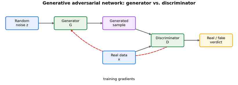
The families so far mostly discriminate — they map an input to a label. A generative model instead learns the distribution of the data well enough to sample new examples from it: fresh images, audio, or text that never existed. Several distinct designs share this goal. The generative adversarial network (GAN) in Fig 7 pits two networks against each other; the variational autoencoder (VAE) and diffusion models take other routes to the same end. The common thread is that they all learn a parametric approximation of the true data distribution, usually by minimising a divergence such as the Kullback–Leibler divergence or the Wasserstein distance, and once trained, they can generate new samples by drawing from a simple prior (e.g., a standard Gaussian) and passing it through the learned generator.
Origins and rise
Goodfellow's GAN in 2014 framed generation as a game between a generator and a discriminator, and for several years produced the sharpest synthetic images available.[72] In parallel, the VAE gave a probabilistic, more stable route to a smooth latent space.[73] The current wave belongs to diffusion models, introduced as DDPM in 2020, which learn to reverse a gradual noising process and generate by denoising pure noise.[74] Moving that process into a compressed latent space produced Stable Diffusion and the text-to-image systems now in wide use.[75] Notably, these generators are not a rival branch of the tree so much as a way of using it: their building blocks are convolutional and Transformer networks turned toward synthesis.
5.1 Generative adversarial networks
The GAN casts generation as a game: a generator turns noise into samples while a discriminator learns to tell them from real data.[72] DCGAN pinned down the convolutional recipe that first made this train reliably,[76] but the objective was notoriously unstable and prone to mode collapse. The Wasserstein GAN reframed the loss around a smoother distance and largely tamed that instability,[77] while self-attention (SAGAN) let the generator model long-range structure across a whole image.[78]
Scale and architecture then chased photorealism. Progressive growing built images coarse-to-fine for the first convincing megapixel faces,[79] StyleGAN's style-based generator gave separate control over coarse and fine attributes and set the bar for face synthesis,[80] and BigGAN scaled class-conditional generation to ImageNet.[81] A second thread mapped one image domain to another: Pix2Pix learned paired translation such as sketch-to-photo,[82] and CycleGAN removed the need for paired data with a cycle-consistency loss.[83] GANs also drove super-resolution — SRGAN and ESRGAN[32] — and audio synthesis (WaveGAN, HiFi-GAN), while text-to-image GANs such as StackGAN and AttnGAN were later overtaken by diffusion.
5.2 Variational autoencoders
The VAE takes a probabilistic route: an encoder maps each input to a distribution in a latent space, and a decoder reconstructs from samples of it, trained to keep that space smooth and continuous.[73] Constraining the latent code — as in β-VAE — encourages disentangled, individually meaningful factors. The most influential branch made the code discrete: VQ-VAE quantises it against a learned codebook, sidestepping blurry reconstructions and pairing naturally with autoregressive or Transformer priors,[84] a design extended by VQ-VAE-2 and NVAE. VQGAN added an adversarial loss on top, and its perceptual latent codes became the compression stage that makes latent diffusion practical.[85]
5.3 Autoregressive models
An autoregressive model factorises data into an ordered product and predicts one element at a time, each conditioned on all before it. For images, PixelRNN and PixelCNN generate pixel by pixel,[86] a line that led to ImageGPT and to the VQ-VAE-plus-Transformer stack behind the first DALL·E. For audio, WaveNet generates raw waveforms sample by sample and reset the bar for speech synthesis,[87] with WaveRNN and SampleRNN trading quality for speed. The approach gives exact likelihoods and stable training, at the cost of slow sequential sampling.
5.4 Diffusion models
Diffusion models, today's dominant image generators, learn to reverse a gradual noising process: corrupt an image with many small steps of Gaussian noise, then train a network to undo each step so that sampling can start from pure noise.[74] DDIM made sampling far faster by turning the reverse process deterministic and skipping steps,[88] while the score-based SDE view unified diffusion with score matching and continuous-time dynamics.[89] The turning point for adoption was the finding that a well-tuned diffusion model beats GANs on image quality.[90]
Moving the process into a VAE's compressed latent space gave latent diffusion — Stable Diffusion — cutting cost enough for consumer hardware,[75] with SDXL scaling it to higher resolution and quality.[91] Cascaded pixel-space systems such as Imagen and DALL·E 2/3 took a parallel path (their text-to-image side belongs to the multimodal family). Because sampling is the bottleneck, fast solvers such as DPM-Solver and consistency models cut the step count from thousands to a handful.[92] The same denoising recipe now drives video (Make-A-Video), 3D (DreamFusion), and speech (DiffWave).
5.5 Flow-based models
A normalising flow builds a generator from a stack of exactly invertible transformations, so it can both sample and compute exact likelihoods — unlike a GAN or VAE. RealNVP introduced the coupling layers that keep the Jacobian tractable,[93] and Glow added invertible 1×1 convolutions for high-quality image synthesis.[94] NICE, Flow++, and FFJORD extend the idea, and rectified flow — which learns straight-line transport between noise and data — has re-emerged at the heart of recent systems such as Stable Diffusion 3.
5.6 Energy-based models
An energy-based model learns a scalar energy that is low on real data and high elsewhere, then samples by descending that landscape — the oldest generative idea here. The restricted Boltzmann machine and the deep belief networks stacked from it were central to the deep-learning revival of the mid-2000s.[7] Modern revivals such as JEM show that an ordinary classifier is secretly an energy-based model and can be trained to generate as well as classify.[95] Sampling remains the hard part, which is why the families above, with their direct sampling paths, now dominate.
Applications
- Text-to-image and image editing, super-resolution, and inpainting.
- Speech and music synthesis.
- Data augmentation and simulation where real examples are scarce.
Strengths and limitations
| Strengths | Limitations |
|---|---|
| Produce novel, high-fidelity samples. | GAN training can be unstable and mode-collapse. |
| Diffusion is stable and covers the data well. | Diffusion sampling is slow, needing many steps. |
| Learn reusable latent representations. | Raise real concerns over misuse and training-data rights. |