6. Graph Neural Networks (GNN)
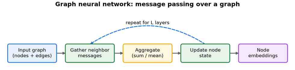
A graph neural network works on data shaped as a graph — nodes joined by edges — rather than a grid or a sequence. It runs on message passing: each node repeatedly gathers information from its neighbours, aggregates it, and updates its own state, as in Fig 8. In effect it generalises the weight sharing of a convolutional network from a regular pixel grid to arbitrary, irregular connectivity. The aggregation function is typically a permutation-invariant operation (sum, mean, or max) to respect the fact that neighbours have no intrinsic order, and the update step is often an MLP that combines the node's own representation with the aggregated message.
Origins and rise
Early work defined convolution in the graph's spectral domain, but the field took off with the simple, scalable graph convolutional network (GCN) of Kipf and Welling in 2017.[96] Graph Attention Networks (GAT) then let each node weigh its neighbours by learned importance — the same idea as the attention modules and Transformer that appear elsewhere in this tree.[97]
Spectral methods
The earliest graph networks borrowed from signal processing, defining convolution through the graph's Laplacian spectrum. ChebNet approximated those spectral filters with Chebyshev polynomials, making them local and cheap to compute,[98] and the GCN simplified this to a single-hop averaging rule that became the field's default baseline.[96] Purely spectral filters are tied to one fixed graph, however, which pushed the field toward the spatial view below.
Spatial message passing
Spatial methods define a layer directly as message passing over neighbours, and most modern GNNs are variants of it. GraphSAGE made the scheme inductive by sampling and aggregating a fixed number of neighbours, so a trained model generalises to unseen nodes and enormous graphs.[99] The message-passing neural network framework then unified many of these designs under one gather-and-update template.[100] GAT weighs neighbours by learned attention,[97] while the graph isomorphism network (GIN) was built to be as discriminative as the Weisfeiler–Lehman test, clarifying exactly how expressive message passing can be.[101] GATv2, PNA, GatedGCN, and EdgeConv (DGCNN) extend the aggregation and edge-handling machinery.
Geometric and higher-order networks
Because plain message passing cannot tell some structures apart, one line adds higher-order information — SubGNN, k-GNNs, and graph substructure networks (GSN) count subgraphs or reason over node tuples. A closely related thread targets molecules and 3D point sets, where geometry matters: SchNet uses continuous-filter convolutions to model atomic interactions,[102] DimeNet and GemNet add directional and angular detail, and SE(3)-Transformers build in rotation and translation equivariance so predictions respect physical symmetry.[103] Equiformer and TorchMD-Net carry the same idea into molecular dynamics.
Spatiotemporal graphs
When a graph also evolves in time — traffic sensors, moving skeletons, sensor arrays — spatiotemporal GNNs combine graph convolution across space with sequence modelling across time. ST-GCN applies this to skeleton-based action recognition,[104] while DCRNN and Graph WaveNet forecast traffic by pairing diffusion or dilated-convolution dynamics with a learned graph structure.[105] MTGNN extends the approach to general multivariate time series.
Graph transformers
As Transformers spread, researchers asked whether attention over all nodes could replace message passing. Graphormer showed it can, encoding graph structure through carefully designed positional and edge biases to win molecular-property benchmarks.[106] GraphGPS offers a modular recipe that mixes local message passing with global attention, and TokenGT, SAT, and Grit explore other ways to feed graph structure to a Transformer.
Self-supervised graph learning
Labels on graphs are often scarce, so contrastive and bootstrapping methods pre-train on structure alone. GraphCL learns representations invariant to graph augmentations such as edge dropping and subgraph sampling,[107] JOAO automates the choice of those augmentations, and BGRL drops the need for negative samples by bootstrapping, scaling self-supervision to very large graphs.
Applications
- Molecular property prediction and drug discovery.
- Recommendation, fraud detection, and social-network analysis.
- Traffic forecasting and physical simulation on meshes.
Strengths and limitations
| Strengths | Limitations |
|---|---|
| Handle arbitrary relational structure. | Deep stacks over-smooth, blurring nodes together. |
| Invariant to node ordering. | Hard to scale to graphs with billions of edges. |
| Reuse one operator across the whole graph. | Sensitive to how the graph itself was built. |