3. Recurrent Neural Networks (RNN)
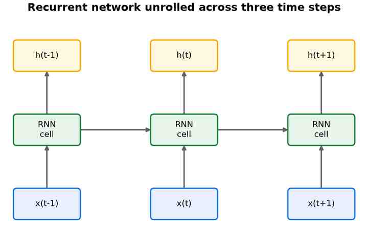
A recurrent neural network processes a sequence one step at a time, keeping a hidden state that carries information forward from earlier steps. The same cell is applied at every step, so the network can handle sequences of any length; drawn “unrolled” in time it looks like Fig 5, with the hidden state passed sideways from one step to the next. This makes the RNN a natural fit for text, audio, and time series. The recurrence can be written as h_t = f(h_{t-1}, x_t), where the same function f and the same weight matrix are reused at every timestep. This weight-tying makes the model compact and, in principle, capable of capturing dependencies of arbitrary length.
Origins and rise
Elman's simple recurrent network in 1990 established the pattern,[34] but plain RNNs suffered the same vanishing-gradient problem as deep feedforward stacks: they forgot information from more than a few steps back. The breakthrough was the long short-term memory (LSTM) cell of Hochreiter and Schmidhuber in 1997, which added a protected memory cell and multiplicative gates that decide what to keep, forget, and output.[35] The gates are computed as sigmoid functions of the current input and previous hidden state, producing values between 0 and 1 that act as soft switches. The cell state passes information almost unchanged across long time spans, which is why LSTMs can retain context over hundreds of steps. The lighter gated recurrent unit (GRU) of 2014 achieved much the same with fewer gates.[36] Through the mid-2010s, gated RNNs powered machine translation, speech recognition, and the first strong language models.
3.1 Simple recurrent networks
The earliest designs simply feed the previous state back as an extra input. Elman's network loops the hidden layer; Jordan's loops the output layer. Both are trained by backpropagation through time (BPTT), which unrolls the loop into a deep feedforward graph and applies ordinary backpropagation. Their habit of forgetting anything more than a few steps back is exactly what the gated cells below were built to cure.
3.2 LSTM and its variants
The LSTM's protected cell spawned a family of tweaks. Peephole connections let the gates read the cell state directly; the bidirectional LSTM runs one pass forward and one backward so every step sees future as well as past context;[37] and stacked and grid LSTMs add depth across layers and dimensions. ConvLSTM swaps the cell's matrix multiplies for convolutions, letting it model spatiotemporal data such as radar maps and video.[38]
3.3 GRU and its variants
The GRU merged the LSTM's forget and input gates into a single update gate. Lighter still are the minimal gated unit, which keeps just one gate, and Light GRU; ConvGRU applies the same convolutional trick as ConvLSTM. In practice GRU and LSTM trade blows, with the GRU often preferred for its smaller state and faster training.
3.4 Efficient recurrent networks
A recurrent cell's step-to-step dependency blocks the parallelism GPUs thrive on, and several designs claw it back. The quasi-recurrent neural network (QRNN) interleaves convolutions with a minimal recurrent pooling step;[39] the simple recurrent unit (SRU) drops the state-to-state matrix so most of the work runs in parallel;[40] and the independently recurrent neural network (IndRNN) makes the neurons within a layer independent, enabling very deep, long-memory recurrence.[41] FastGRNN and Delta RNN target tiny, on-device budgets.
3.5 Memory-augmented networks
Some tasks need an addressable memory far larger than a hidden state. The neural Turing machine (NTM) couples a recurrent controller to an external memory it reads and writes through differentiable attention;[42] its successor, the differentiable neural computer (DNC), added dynamic memory allocation and could answer graph and reasoning questions.[43] End-to-end memory networks stack several soft-attention lookups over a stored set of facts — a direct ancestor of the attention that would soon eclipse recurrence entirely.[44]
3.6 Reservoir computing
Reservoir computing takes the opposite tack: leave the recurrent weights fixed and random, and train only a linear readout on top. The echo state network does this with a rate-based reservoir,[45] while the liquid state machine uses a pool of spiking neurons;[46] next-generation reservoir computing reproduces the effect with an explicit polynomial feature map. Cheap to train, these models shine at chaotic time-series prediction.
Applications
- Speech recognition and text-to-speech.
- Time-series forecasting and anomaly detection.
- Streaming and on-device tasks where inputs arrive one step at a time.
Strengths and limitations
| Strengths | Limitations |
|---|---|
| Handle variable-length sequences naturally. | Sequential processing cannot be parallelised across time. |
| Compact state, well suited to streaming. | Still struggle with very long-range dependencies. |
| Gated cells tame the vanishing gradient. | Slow to train on long sequences. |
That first limitation — the step-by-step bottleneck that stops an RNN from using modern hardware fully — is what the Transformer was designed to eliminate, and its removal reshaped the entire field.