20. Deep Equilibrium Models
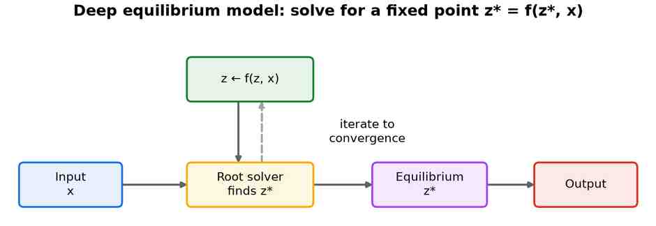
A deep equilibrium model (DEQ) replaces a deep stack of layers with a single layer applied until it settles to a fixed point, where the output stops changing: z* = f(z*, x). As Fig 22 shows, a root-finding solver drives the iteration, and gradients come from implicit differentiation at the solution — so training uses constant memory no matter the effective depth.
Origins and rise
Bai, Kolter & Koltun introduced DEQs, showing a single implicit layer can match a deep weight-tied network.[291] Multiscale DEQ extended the idea to several resolutions at once, reaching competitive results on image classification and language modelling.[292] Like neural ODEs, DEQs treat depth implicitly rather than as a fixed stack of layers.
Guaranteeing and stabilising equilibria
An implicit layer is only useful if its fixed point exists, is unique, and can be found reliably. Implicit Deep Learning set out the general framework, giving well-posedness conditions under which an equilibrium equation defines a valid layer.[293] Monotone operator equilibrium networks made this constructive: by parameterising the layer as a monotone operator, they guarantee a unique fixed point reachable by a provably convergent solver.[294] In practice DEQs can grow unstable as training proceeds, so Jacobian regularisation penalises the fixed-point Jacobian to keep the solver fast and the model well-conditioned.[295]
Implicit models across domains
The equilibrium idea travels well beyond sequence models. Implicit graph neural networks solve for a fixed point of the message-passing update, behaving like an infinitely deep GNN that captures long-range dependencies a few explicit layers miss.[296] Deep equilibrium optical flow solves directly for the flow field as the fixed point of an implicit refinement layer, matching recurrent estimators at a fraction of the training memory.[297] This continuous, memory-light view of depth is shared with neural ODEs, which reach a solution by integrating a differential equation rather than by finding a fixed point.[136]
Applications
- Memory-constrained sequence and vision models.
- Implicit graph neural networks.
- Very-deep behaviour without storing every layer.
Strengths and limitations
| Strengths | Limitations |
|---|---|
| Constant training memory at any effective depth. | Each forward pass runs an iterative solver. |
| Backprop needs only the fixed point. | Convergence is not guaranteed. |
| Elegant and expressive. | Slower and less stable than explicit stacks. |