26. Optical, Analog & Unconventional Networks
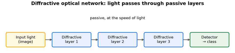
Not every neural network runs on a digital processor. Unconventional hardware performs the computation physically: a diffractive optical network, in Fig 28, sends light through a stack of passive, patterned layers whose interference implements the “weights,” and detectors read out the answer — inference at the speed of light with almost no power draw.
Origins and rise
Lin et al. built an all-optical diffractive deep neural network that classifies images passively.[338] Shen et al. demonstrated a programmable nanophotonic processor performing matrix multiplication with interferometers.[339] Related analog approaches use in-memory crossbar arrays and physical reservoirs, echoing the energy-efficiency goals of spiking networks.
Optical and photonic networks
Light computes convolutions at the speed of propagation. The diffractive deep neural network (D²NN) lays out successive diffractive optical layers and trains their phase masks so that the transmitted light pattern performs inference at the speed of light.[338] Integrated photonic circuits carry the same idea onto a chip, using Mach-Zehnder interferometer meshes to perform matrix multiplication optically for low-energy inference.[339]
Analog in-memory computing
Memristive crossbar arrays store weights as conductance levels and perform matrix-vector multiplication in a single analogue step by Kirchhoff's laws, making them natural for neuromorphic and edge inference. The trade-off is limited precision, device variability, and the difficulty of on-chip training, which is why most analogue arrays ship as accelerators for a frozen digital model.
Physical reservoir computing
A reservoir — any high-dimensional dynamical system — can serve as a fixed random feature map, leaving only a linear readout to be trained. Beyond the echo-state networks already discussed, researchers have built reservoirs from optical cavities, mechanical oscillators, and spintronic devices, exploiting their natural dynamics to classify temporal signals with minimal training energy.
Applications
- Ultra-low-power, low-latency inference.
- Optical front-ends for imaging and sensing.
- Edge accelerators for fixed models.
Strengths and limitations
| Strengths | Limitations |
|---|---|
| Extremely fast, energy-efficient inference. | Fabrication fixes the weights; hard to retrain. |
| Massively parallel by physics. | Analog noise and calibration drift. |
| No digital multiply-accumulate. | Limited to specific, mostly linear operations. |