10. Neural Differential Equations
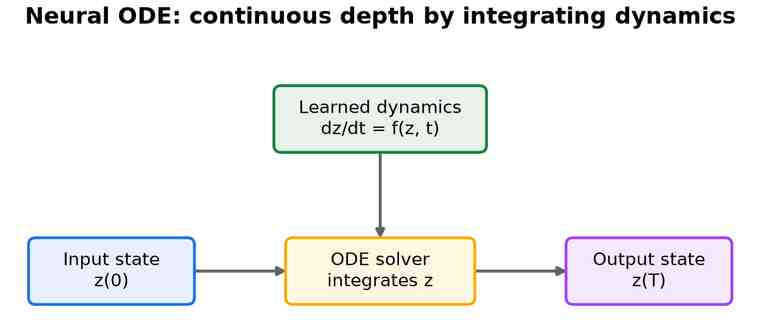
A neural ordinary differential equation (ODE) treats network depth as continuous. Instead of stacking a fixed number of discrete layers, it defines how the hidden state changes — its derivative — and hands that to an ODE solver to integrate from input to output, as in Fig 12. A residual network turns out to be a coarse, discrete version of exactly this — one Euler step per layer. The ODE formulation provides a natural way to adapt the number of function evaluations to the complexity of the problem, a property known as adaptive computation.
Origins and rise
Chen and colleagues introduced neural ODEs in 2018, training them memory-efficiently by solving a second, adjoint equation backwards.[136] The framework extends naturally to continuous-time data and to generative normalising flows, and it links deep learning to a century of numerical-analysis tools.
Continuous-depth models and their limits
The original neural ODE recast a deep stack as the integral of a learned vector field,[136] but that continuity carries a catch: because ODE trajectories cannot cross, a single neural ODE cannot represent some mappings a residual network handles with ease. Augmented neural ODEs resolve this by adding extra dimensions to the state, giving the trajectories room to flow around one another, which improves both expressivity and training stability.[137]
Continuous-time models for irregular data
A key payoff of the framework is native handling of data that arrives at irregular times, where discrete recurrent networks must awkwardly bin or interpolate. Latent ODEs pair a recurrent encoder with an ODE that evolves a latent state in continuous time, so an observation at any timestamp slots in naturally.[138] Neural controlled differential equations go further, driving the dynamics with an interpolated path of the incoming data — a continuous-time analogue of the RNN that inherits the mathematics of controlled differential equations and copes gracefully with partially observed streams.[139]
Stochastic dynamics and continuous flows
The same machinery reaches from deterministic ODEs into probability and randomness. FFJORD turns a neural ODE into a continuous normalising flow, using an unbiased trace estimator so that exact likelihoods can be computed without the architectural constraints earlier flows imposed.[140] Replacing the ODE with a stochastic differential equation adds a noise term: neural SDEs learn both a drift and a diffusion, trained with an adjoint sensitivity method that scales to many parameters,[141] and casting such an SDE as the generator of a GAN yields a principled continuous-time generative model for time series.[142]
Applications
- Irregularly sampled time series and continuous-time modelling.
- Continuous normalising flows for generative modelling.
- Physics- and dynamics-aware scientific models.
Strengths and limitations
| Strengths | Limitations |
|---|---|
| Constant memory via the adjoint method. | The ODE solver makes training slow. |
| Adapt computation to the problem's difficulty. | Can be numerically stiff or unstable. |
| Natural fit for continuous-time data. | Often outperformed by simpler nets on plain tasks. |