7. Self-Organizing Maps (SOM) & Competitive Learning
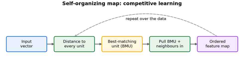
A self-organizing map is an unsupervised network that projects high-dimensional data onto a low-dimensional grid while preserving its topology: similar inputs end up near each other on the map. It learns by competition rather than backpropagation — for each input the closest unit “wins” and is nudged, along with its neighbours, toward that input, as Fig 9 shows. This makes it a very different animal from the backprop-trained feedforward networks that dominate the rest of this tree. The neighbourhood radius is typically annealed over training, starting large to form a global ordering and shrinking to refine local details.
Origins and rise
Kohonen introduced the map in 1982, and it became a staple of exploratory data analysis and visualisation through the 1990s.[108] Related competitive schemes — learning vector quantization, neural gas, growing networks — share the winner-take-all idea. For modern representation learning the family has largely been overtaken by the self-supervised metric-learning methods discussed later.
The Kohonen map and its variants
Kohonen's original map fixes a rectangular or hexagonal grid of units and adapts them to the data.[108] Because computing every winner online is slow, the batch SOM updates all units together in one sweep, and hierarchical variants stack maps for coarse-to-fine structure. The growing hierarchical SOM (GHSOM) removes the need to fix the grid in advance, expanding both the size of each map and the depth of the hierarchy to match the data's complexity.[109]
Growing and topology-learning networks
A related family drops the fixed grid entirely and lets the network's own graph grow to fit the data. Neural gas sorts all units by their distance to each input and adapts them in that order, learning a topology without any predefined layout.[110] Growing neural gas (GNG) and its utility-driven GNG-U variant add and delete units and edges on the fly, while growing when required (GWR) inserts a new unit whenever the existing ones fit an input poorly, which suits non-stationary data.[111] The topology-representing network formalises the edges these methods learn as an induced Delaunay graph.
Learning vector quantization
Where the maps above are unsupervised, learning vector quantization (LVQ) is their supervised cousin: it places labelled prototypes in the input space and, for each training example, pulls the nearest correct prototype closer and pushes wrong ones away. Kohonen's LVQ1/2/3 set the pattern, and later work made it principled — generalized LVQ (GLVQ) optimises a differentiable cost, while GRLVQ and RSLVQ add learned feature relevances and a probabilistic formulation.[112] The result is a compact, interpretable nearest-prototype classifier.
Applications
- Visualising and clustering high-dimensional data.
- Vector quantization and data compression.
- Exploratory analysis in finance, genomics, and process monitoring.
Strengths and limitations
| Strengths | Limitations |
|---|---|
| Unsupervised; needs no labels. | Fixed grid size and shape set in advance. |
| Produces an interpretable 2D map. | Does not scale to today's large, complex tasks. |
| Preserves topology of the data. | Largely superseded for feature learning. |