18. Temporal Convolutional & Time-Series Networks
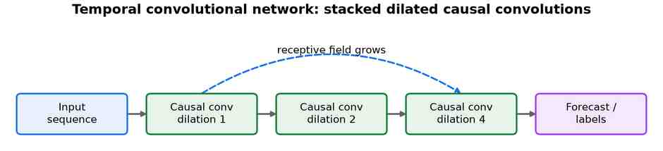
Sequences do not have to be processed with recurrence. A temporal convolutional network (TCN) stacks dilated causal convolutions, shown in Fig 20, whose receptive field grows exponentially with depth — so each output can look far into the past while, unlike an RNN, every time step is computed in parallel.
Origins and rise
Bai, Kolter & Koltun showed that a generic TCN matches or beats LSTMs across a wide range of sequence benchmarks.[269] For forecasting specifically, N-BEATS stacked fully connected blocks with a basis-expansion structure,[270] and Informer made the Transformer efficient for long-horizon time series with a sparse attention mechanism.[271]
Dilated-convolution forecasters
The dilated causal stack that defines the TCN predates it: WaveNet introduced dilated causal convolutions to generate raw audio sample by sample, and the same structure underlies the general-purpose TCN.[87] SCINet refines the convolutional route for forecasting: it repeatedly downsamples the series into odd and even sub-sequences and lets them interact, so each convolution sees several temporal resolutions at once.[272]
Specialised forecasting networks
A line of purpose-built forecasters extends the basis-expansion idea of N-BEATS.[270] N-HiTS adds multi-rate sampling and hierarchical interpolation, cutting the cost of long-horizon forecasts while improving accuracy.[273] Where those give point forecasts, DeepAR trains an autoregressive recurrent network to output the parameters of a probability distribution, producing calibrated uncertainty across thousands of related series.[274] MQRNN instead predicts a set of quantiles directly for every future step, giving multi-horizon prediction intervals in a single pass.[275] Temporal Fusion Transformer combines recurrent encoding, variable-selection networks, and interpretable attention to mix static, known-future, and observed inputs in one model.[276]
Transformers for long-horizon forecasting
After Informer made long-range attention tractable,[271] a wave of Transformer forecasters targeted the structure of time series directly. Autoformer replaces dot-product attention with an auto-correlation mechanism and an internal series-decomposition block,[277] and FEDformer moves the mixing into the frequency domain for a linear-complexity attention.[278] PatchTST showed that splitting each channel into sub-series patches and treating channels independently gives a simple, strong baseline,[279] while TimesNet reshapes a 1-D series into 2-D tensors along discovered periods so ordinary convolution captures both intra- and inter-period variation.[280]
Time-series anomaly detection
Detecting anomalies in multivariate telemetry is usually framed as unsupervised reconstruction: a model learns normal dynamics and flags what it cannot reproduce. USAD pairs two autoencoders in an adversarial game so reconstruction is sensitive to subtle deviations,[281] TranAD uses a lightweight Transformer with adversarial training and fast meta-learning to score deviations across many channels,[282] and the Anomaly Transformer exploits an association-discrepancy criterion — anomalies attend locally while normal points attend globally — to separate the two.[283]
Applications
- Demand, energy, and financial forecasting.
- Anomaly detection in sensor and system telemetry.
- Long causal sequences where parallel training matters.
Strengths and limitations
| Strengths | Limitations |
|---|---|
| Parallel training with stable gradients. | Receptive field is fixed at design time. |
| Long memory through dilation. | Long horizons need many layers or wide kernels. |
| A simple, strong forecasting baseline. | Less flexible than attention for irregular sampling. |