11. Spiking Neural Networks (SNN)
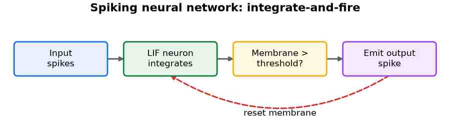
A spiking neural network is the family closest to the biology the introduction invoked. Its neurons communicate not with continuous numbers but with discrete spikes over time: a LIF neuron integrates incoming spikes until its membrane potential crosses a threshold, fires a spike, and resets, as in Fig 13. Computation is therefore sparse and event-driven. The dynamics of a LIF neuron can be described by the differential equation τ dV/dt = - (V - V_rest) + R I(t), where V is the membrane potential, τ is the time constant, and I(t) is the input current. When V exceeds a threshold, a spike is emitted and the potential resets.
Origins and rise
Maass framed spiking neurons as a “third generation” of network models in 1997.[143] Because a spike is not differentiable, training was long the obstacle; the modern answer is the surrogate gradient, which substitutes a smooth approximation during backpropagation.[144] Interest has grown alongside neuromorphic hardware, and many spiking models are obtained by converting a trained convolutional network.
Neuron models
How faithfully a spiking neuron mimics biology is a design choice. The leaky integrate-and-fire neuron of Fig 13 keeps only the essentials — leak, integrate, threshold, reset — and dominates practical work for its simplicity. The Izhikevich model adds a second recovery variable and, for only a handful of operations per step, reproduces the rich firing patterns of cortical neurons: bursting, chattering and adaptation.[145] The adaptive exponential integrate-and-fire (AdEx) neuron sits between the two, pairing an exponential spike-initiation term with an adaptation current, and matches real recordings closely enough to serve as a workhorse in large-scale simulations.[146]
Spike-timing-dependent plasticity
The oldest way to train a spiking network borrows a rule from neuroscience: spike-timing-dependent plasticity (STDP) strengthens a synapse when a presynaptic spike arrives just before a postsynaptic one and weakens it otherwise, learning from local timing alone with no global error signal. Diehl and Cook showed that a two-layer network trained this way, entirely unsupervised, recognises handwritten digits at competitive accuracy — an existence proof that biologically local learning scales beyond toy problems.[147] Its appeal is hardware-friendliness — the update is local and needs no backward pass — but it has been hard to push to the depths gradient training reaches.
Converting trained networks to spikes
A pragmatic shortcut sidesteps spiking training altogether: train an ordinary convolutional network with real-valued activations, then convert it into a spiking one whose firing rates approximate those activations. Rueckauer and colleagues formalised the recipe — rescaling weights and thresholds so a rate-coded spiking network matches the original's accuracy — and extended it to the operations, such as max-pooling and batch normalisation, that real networks depend on.[148] Sengupta and colleagues then scaled conversion to deep VGG and residual networks on ImageNet, closing much of the accuracy gap to the source model.[149] Conversion buys accuracy at the price of latency, since firing rates need many timesteps to settle.
Surrogate-gradient training and deep spiking networks
Training a spiking network directly means confronting the non-differentiable spike, and the modern answer — the surrogate gradient introduced above — replaces the threshold's derivative with a smooth stand-in so that backpropagation through time can flow.[144] SLAYER made this practical by also distributing the credit for an error backwards across time, accounting for a spike's delayed influence on the ones that follow.[150] Scaling the idea deep required taming the firing statistics: a threshold-dependent batch normalisation let directly trained networks reach residual depths without the signal vanishing or saturating.[151] Spikformer carried the approach into the Transformer era, recasting self-attention in a purely spike-driven, multiplication-free form.[152]
Recurrent spiking networks and neuromorphic hardware
Because spikes unfold in time, a spiking network is inherently recurrent, and adding explicit feedback plus slow adaptation yields memory rivalling an LSTM: the LSNN equips neurons with an adapting threshold and learns tasks that demand holding information across many timesteps.[153] The payoff for all this is energy, realised on neuromorphic hardware that computes only when spikes occur. IBM's TrueNorth packed a million spiking neurons onto a chip drawing tens of milliwatts,[154] and Intel's Loihi added on-chip plasticity so that STDP-style learning can run in silicon.[155] These chips are the reason the family is pursued despite trailing standard networks on raw accuracy.
Applications
- Ultra-low-power inference on neuromorphic chips such as Loihi and TrueNorth.
- Event-camera and always-on sensing at the edge.
- Computational-neuroscience models of the brain.
Strengths and limitations
| Strengths | Limitations |
|---|---|
| Very energy-efficient on neuromorphic hardware. | Non-differentiable spikes are hard to train. |
| Naturally encode timing and events. | Tooling and hardware are still immature. |
| Biologically plausible. | Often trail standard networks on accuracy. |